Hash table

A hash table is a data structure that implements the interface of an associative array, namely, it allows you to store pairs (key, value) and perform three operations: the operation to add a new pair, the search operation, and the operation to delete the pair by key.

Introduction

There are two main options for hash tables: with chains and open addressing. The hash table contains some array elements of which are pairs (hash table with open addressing) or lists of pairs (hash table with chains).

The operation in the hash table begins with the calculation of the hash function from the key. The resulting hash value plays the role of the index in the array . Then the performed operation (add, delete or search) is redirected to the object, which is stored in the corresponding cell of the array .

The situation when the same hash value is obtained for different keys is called a collision. Such events are not so rare - for example, when inserting only 23 elements into a hash table of 365 cells in size, the probability of a collision already exceeds 50% (if each element can be equally likely to fall into any cell) - see the paradox of birthdays. Therefore, the collision resolution mechanism is an important component of any hash table.

In some special cases, it is possible to avoid collisions altogether. For example, if all the keys of the elements are known in advance (or very rarely change), then you can find some perfect hash function for them, which will distribute them among the hash table cells without collisions. Hash tables using similar hash functions do not need a collision resolution mechanism, and are called directly addressed hash tables.

The number of stored items divided by the size of the array (the number of possible hash values) is called the load factor of the hash table (load factor) and is an important parameter on which the average execution time of operations depends.

Hash Table Properties

An important property of hash tables is that, with some reasonable assumptions, all three operations (search, insert, delete items) are performed on average over time. . But it is not guaranteed that the execution time of a single operation is short. This is due to the fact that when a certain value of the fill factor is reached, it is necessary to reorganize the hash table index: increase the value of the array size and re-add all pairs to the empty hash table.

Conflict Resolution

There are several ways to resolve collisions.

Chaining Method

Collision resolution using chains.

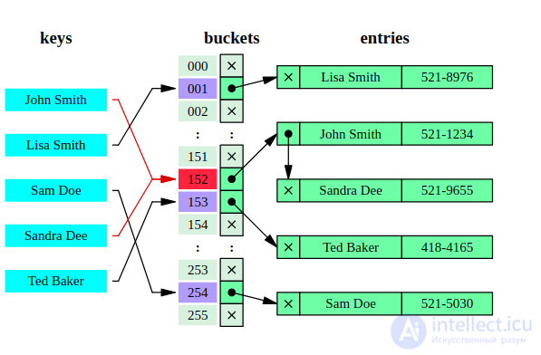
Each cell of the array H is a pointer to a linked list (chain) of key-value pairs corresponding to the same key hash value. Collisions simply lead to the fact that there are chains with a length of more than one element.

Operations of searching or deleting an element require viewing all the elements of the corresponding chain in order to find an element with a given key in it. To add an element, you need to add an element to the end or the beginning of the corresponding list, and if the fill factor becomes too large, increase the size of the array H and rebuild the table.

Assuming that each element can fall into any position of the table H with equal probability and regardless of where any other element is, the average operation time of the element search operation is Θ (1 + α ), where α is the fill factor of the table.

Open Addressing [edit]

An example of a hash table with open addressing and linear probing, resulting from the insertion of elements in the left column from top to bottom.

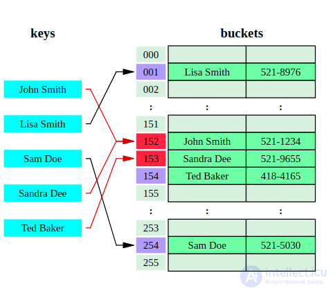
The H -key pairs themselves are stored in the array. The element insertion algorithm checks the cells of the array H in a certain order until the first free cell is found, in which the new element will be written. This order is calculated on the fly, which saves memory for pointers required in chained hash tables.

The sequence in which the hash table cells are viewed is called a sample sequence . In general, it depends only on the key of the element, that is, it is the sequence h ₀ ( x ), h ₁ ( x ), ..., h _{n - 1} ( x ), where x is the key of the element, and h _i ( x ) - arbitrary functions that associate each key with a cell in the hash table. The first element in the sequence, as a rule, is equal to the value of a certain hash function of the key, and the rest are considered from it in one of the following ways. For successful operation of the search algorithms, the sequence of samples must be such that all the cells of the hash table are scanned exactly once.

The search algorithm scans the hash table cells in the same order as they were inserted, until either an element with the desired key or a free cell is found (which means the absence of an element in the hash table).

Removing elements in such a scheme is somewhat difficult. Usually they do this: they turn on a boolean flag for each cell, which marks whether the element is removed in it or not. Then deleting an element consists in setting this flag for the corresponding hash table cell, but at the same time it is necessary to modify the search procedure of the existing element so that it considers the deleted cells to be occupied, and the addition procedure - so that it considers them free and resets the flag value when added.

Sample sequences

Below are some common types of sample sequences. We will immediately stipulate that the numbering of the elements of the sample sequence and the hash table cells is zero, and N is the size of the hash table (and, as noted above, also the length of the sample sequence).

• Linear probing: hash table cells are sequentially scanned with a fixed interval k between cells (usually, k = 1), that is, the i- th element of the sample sequence is the cell with the number (hash ( x ) + ik ) mod N. In order for all cells to be scanned once, it is necessary that k be mutually simple with the size of the hash table.
• Quadratic probing: the interval between cells with each step increases by a constant. If the size of the hash table is equal to the power of two ( N = 2 ^p ), then one of the examples of the sequence in which each element will be viewed once is:

  hash ( x ) mod N , (hash ( x ) + 1) mod N , (hash ( x ) + 3) mod N , (hash ( x ) + 6) mod N , ...

• Double hashing: the interval between cells is fixed, as in linear probing, but, unlike it, the size of the interval is calculated by the second, auxiliary hash function, and therefore may be different for different keys. The values ​​of this hash function should be non-zero and mutually simple with the size of the hash table, which is easiest to achieve by taking a prime number as a size, and requiring the auxiliary hash function to take values ​​from 1 to N - 1.

Below is a code that demonstrates double hashing: