Lecture
"Table
Multiplications
Worthy of
Respect
C.Y. Marshak
"Show me the flowcharts, not showing the tables, and I will be confused. Show me your tables, and the flowcharts will most likely not be needed: they will be obvious."
Frederick Brooks
Turn again to our model object - the multiplication table. Obviously, the standard dimensions of this structure - 10 × 10 - are dictated by the number system used. Moving to another base, say, to a 16-tier system, will require, first, expanding the table in two directions, and second, initializing new elements (of course, using the old table).
There is a problem of allocating space in the memory for the structure. Well as, it is asked, add 6 rows to the table in fig. A4-3 If the text is on paper, then, as they say, "written in pen ...". The same can be said about the data structure in the program, if the description specifies fixed dimensions. The conclusion is this: the prospect of expanding the living space for the program must be planned in advance, at the design stage of the algorithm. No wonder the sad experience of history shows that most of the wars began because of territorial disputes.
Fortunately, the algorithms and, following it, the computer architecture provide the ability to increase / decrease the size of certain structures during the run-time cycle of their life. The structures of data that allow such manipulations are called dynamic , contrasting them with immutable, - of course, only in size, not content, - static structures . In the formulation of the problem, it is not necessary to have a direct indication of which type of structure is preferred, and the choice is up to the algorithmist.
|
If the reader has not yet had to deal with dynamic structures in his programming practice, then it is desirable to eliminate this gap and get acquainted with the corresponding constructions of the programming language. |
Sometimes it happens in books on computer science to read about the insertion of elements into a static table, but you should not take it at face value. It is either about replacing the values of elements in the filled positions of the table, or about initializing the positions of unfilled ones.
So, anticipating an appeal to the problem "15 × 26", instead of the usual multiplication table, you can pre-allocate space for the table corresponding to the A4-4 algorithm (Fig. A4-4), and initialization can be performed only for the standard size, that is, the upper left corner 10 × 10. In this situation, the dimensions are pre-set "with a stock", and it remains to initialize the rest. The process of "inserting" lines between previously placed ones threatens to become more laborious. It will require moving the row row down, which means, strictly speaking, simply rewriting the elements into new positions, and only then initializing the elements of the "inserted" line. What is, in the same context, the "removal" of elements of a static structure, the reader can easily guess himself.
Completely different, and much more efficiently, the insert algorithms and the removal algorithms for dynamic structures work. Part of Chapter D is devoted to their discussion, and the matter will not be limited to it.
|
What is the complexity of "deleting" k bottom lines in the static placement of the multiplication table m × n ? |
And now let's imagine again the multiplication table of standard sizes, but non-standard content. Let's say we “scattered” the rows of a regular table, and then “collected” them in a random order .
How, technically, to initialize a random order of strings - in our case, natural numbers from 1 to 9? Programming languages, as a rule, provide built-in tools for this, such as the Random function known to the reader. There are many tasks that can be solved by using random number sequences, for example, some cryptography problems, where the ability (or impossibility) of reproducing a sequence that was used to encrypt a message is at the center of attention of the algorithmist. Another example is described in the following exercise.
|
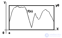
In Lesson A3, you already got acquainted with approximate methods for calculating the integral. The idea of the Monte Carlo method competing with the mechanisms described there will now be illustrated with the same example of calculating the S figure area of a figure bounded above by a graph of a finite, continuous and nonnegative function f (x) , below by a finite interval of the x -axis [a, b] , on the sides - ordinates at the ends of the interval (Fig. A5-1). The figure of interest to us can be completely placed inside a rectangle whose area is limited to the same interval, the same ordinates and some y 0 value majorizing the given function. Now we will alternately launch “a sufficiently large number of times” ( N ) random number sensors to generate points with coordinates from the interval [a, b] and the interval [0, y 0 ] . Accordingly, you can keep track of how many points ( N inside ) "got" inside the shape, and how many are left outside, but, of course, inside the rectangle. At the end of the experiment, the larger the N and the “better” the sensor, the closer to equality the approximate ratio N inside / N≈ S figure / S rectangle . The reader is invited to write the appropriate program and test it for the "table" functions, comparing the results with the values calculated from the integral table. Also of interest is a comparative analysis of the results of calculations using the Monte Carlo method and the methods of rectangles (trapezium and the like) (Fig. A5-1).
|
So, the ability to quickly obtain numbers that make up some random (correct to say: pseudo-random ) sequence is quite relevant. Usually such sets are not stored in the programming system, especially in the operating system, and, if necessary, resort to special algorithms for generating random numbers . We have included an example of constructing such a set in the following exercise.
|
An arbitrary two-digit number is selected and assigned the first element of the n 1 sequence of pseudo-random numbers, and then each successive element n i + 1 is obtained from the previous element n i . To do this, n i is squared, and the left and right numbers are discarded from the four-digit result obtained. For example: n i = 25⇒n i = 0625⇒ n i + 1 = 62 . Since there are a finite number of different numbers in such a sequence, then, sooner or later, it will start reproducing itself starting from a certain place. Therefore, the algorithm generates exactly pseudo-random numbers. Write a program that generates such a sequence for a given input value n 1 . Find the place of the first repeat of the previously received item. |
Let us return to the problem of the "spoiled" multiplication table. Suppose for definiteness that the data storage option turned out to be the same as that shown in Fig. A5-2. Note that the columns, according to the condition, "not affected." How to search for a 5 × 6 product in a “broken” table (fig. A5-2)?
|
||||||||||||||||||||||||||||||||||||||||||||||||||||||||||||||||||||||||||||||||||||||||||||||||||||
| Fig. 2 |
It is impossible to address - by index - directly to the line we need, which was the 5th, because it could move. You have to iterate through the lines one by one, the easiest way is from the top down. To distinguish the desired line from the rest allows its key, located in the left column. Comparing the key value with the first of the factors, only if they coincide, you can further move to the right along the found string. If you shuffle the columns, then the task risks becoming insoluble.
|
System shells Norton Commander , Far , Windows Commander provide the ability, depending on the purpose of use, to change the order of the directory and file names in the Left and Right panels that they display on the screen. Information on these panels comes from the relevant directories of the operating system. Recall (or find out) how directories are organized, what records they consist of, and which fields act as keys. |
What happens if you remove a column and a row with keys from the second, “corrupted” table, as in fig. A5-3? Will the ability to search for all the same 5 × 6 work be preserved?
|
|
Yes, and moreover - you can continue to experiment with the table, and “spoil” it so much that only the first column will remain in it (fig. A5-4), but the possibility of its full restoration will remain. This is because the neighboring elements within each line represent the increasing amounts of the repeating term (remember algorithm A4-1 and Fig. A4-1), and each line contains its own term in it - as the first element.
In other words, we are dealing with the dependence s i, j + 1 = s i, j + s i, 1 , where i is the row number in fig. A5-3 and A5-4, j is the column number in fig. A5-3, s i, j - table element at the intersection of the i- th row and j- th column. Relations of this type are called recurrent . They find application in a variety of tasks, including those related to the processing of tables. The methods and tasks arising in this connection are referred to as the so-called. dynamic programming . They are devoted to Chapter G.
An alternative to methods of dynamic programming based on the use of tables in an explicit form is the use of recursive mechanisms. The use of recursion in a number of tasks and the data structure necessary for this mechanism — the stack — will be discussed in Chapter J.
And again we return to the usual form of the multiplication table. The inverse problem related to the establishment of an “address” in it for a given element value looks quite natural: “for a natural number n, find out at the intersection of which row and column it is recorded”. By the way, if the element is not in the table, the address will not be found.
A non-computer related analogy comes to mind related to the identification of the owner of the keys found near an apartment building. Most likely, the search for an apartment and the owner will have to be carried out sequentially: from the entrance (column of the table) to the entrance, and inside the next entrance - by floors (lines). If the house is large, then the process, the complexity of which is comparable to the number of apartments, can be delayed, and the enthusiasm runs out.
Fortunately, to solve our problem, we can offer more economical algorithms, namely, decompose the input value into various pairs of factors and test them. So, for n = 30 there are several pairs of candidates: (1, 30) , (2, 15) , (3, 10) , (5, 6) , (6, 5) , (10, 3) , (15 , 2) and (30, 1) . Couples including numbers greater than 9 are eliminated immediately. Accordingly, only (5, 6) and (6, 5) remain. In other words, instead of the search algorithm, some computational mechanism is used.
In this example, when the allowed range is limited by the narrow frames of our table, the problem is simply solved "in mind". But as n grows, the problem becomes more complicated and it is desirable to resort to some effective mechanism. Part of us will help out - probably familiar to you - the Euclidean algorithm . He and some related examples are addressed in Chapter C.
Along the way, let us take advantage of the situation and again remind the reader of the “bad” tasks, for the solution of which algorithms of polynomial complexity have not been found. Such, unfortunately, is the problem of decomposing a natural number into prime factors . However, perhaps, "fortunately", the question is how to look. Tasks of this kind find application in cryptography, and, from the point of view of the owner of the secret code, this is good, the spy thinks otherwise.
In our reasoning, we have already changed the data structure several times designed to represent multiplication tables. Most often this was dictated by the desire to reduce the capacitive complexity of the algorithm, allocating less space for data storage. If, at the same time, the aim is not to lose the data, this is precisely the question that arose during the transition from the representation of a picture. A5-3 to fig. A5-4, - then a possible approach would be to establish a one-to-one (element -by- element) correspondence between different representations. Then we can move from one structure to another without affecting the contents of the data set. Approximately according to this scheme, apartment exchange is carried out.
It is convenient if the transition from one structure to another can be described by one formula. But often such transformations are implemented by a multi-step algorithm . Consequently, when replacing the "user structure" with the data structure in a computer program, you should take into account the overhead - machine time - for the implementation of the conversion algorithm . Note that the temporal complexity of such a one-way conversion may differ markedly with the inverse transformation.
We have already seen that the space occupied by the multiplication table is redundant , and it is quite possible to save it using alternative structures. Here is another feature implemented by a multi-step algorithm:
The table is symmetric with respect to the main diagonal (the diagonal going from the upper left to the lower right). Consequently, it is possible, without prejudice to the content, to refuse to allocate space for the lower left triangle of the original square matrix .
Then, line by line, we rewrite what's left in the linear array. The difference between the new representation and the usual storage of a two-dimensional array in RAM is determined by the fact that the truncated lines have different lengths.
Thus, we packaged the source table into a linear array, reducing the capacitance complexity by about half.
|
Build a formula for direct addressing to an element of a packed table view at a given address of the original view, that is, a pair (row_number, col_number). |
|
Build a formula for reverse addressing. |
| Task 1. Multiplication Table (Submit) | ||||||
|
||||||
|
Write a program that, given the N × N multiplication size specified at the input, displays the contents of the upper triangular matrix packed into a linear array, without forming an intermediate set - the table itself. Input Format The first line of the input file contains a single number - N ( 1 <= N <= 1000 ) Output format The output file must contain the resulting array. Numbers must be separated by spaces or line breaks.
|
| Task 2. Reverse multiplication table (Submit) | ||||||
|
||||||
|
Write a program that performs the conversion inverse to the previous task. Input Format The first line of the input file contains a linear array. Numbers are separated by spaces and / or line breaks. The number of numbers does not exceed 1000. Output format The output file must contain the resulting number.
|
The possibility of packing, to which we resorted in the cases considered, was determined by the fact that the data in the table are subject to the above recurrence relation. It is difficult to carry out similar manipulations with the table that we used to “study English numerals” (Lesson A4) if you allocate for the names exactly as much space as each character string takes without aligning their representations in length. However, the problem is solvable if one of the known text compression algorithms is used to package the lines.
A broader formulation of the problem of coding and data compression is presented in Chapter N. In particular, we have to consider various codes : constant length and variable length , and, in connection with the latter, a whole family of Huffman algorithms .
Immediately we draw the attention of the sophisticated reader that we limit ourselves in our course to lossless compression algorithms and it is not worth looking for a description of modern algorithms for packaging video and audio files in this chapter. But to the less sophisticated - we will clarify that we will only deal with such a packaging of information, when the inverse transformation allows restoring “everything as it was”.

Comments
To leave a comment
Structures and data processing algorithms.
Terms: Structures and data processing algorithms.