Lecture
Search is one of the main operations in the processing of information in computers. Its purpose is to find among the data array the data that correspond to this argument by the given argument.
The data set (any) will be called a table or file. Any given (or structure element) differs in some way from other data. This feature is called a key. The key can be unique, that is, there is only one data in the table with this key. This unique key is called primary. The secondary key in one table can be repeated, but it is also possible to organize a search by it. Data keys can be collected in one place (in another table) or be a record in which one of the fields is a key. Keys that are allocated from a data table and organized into their own file are called foreign keys. If the key is in the record, then it is called internal.
A search for a given argument is an algorithm that determines the matching of a key with a given argument. The result of the search algorithm may be finding this data or the absence of it in the table. In the absence of this, two operations are possible:
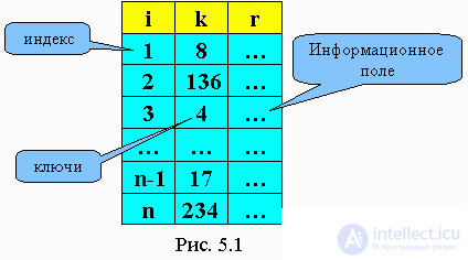
Let k be an array of keys. For each k (i), there is r (i) - given. Key is a search argument. It corresponds to the information record rec. Depending on the data structure in the table, there are several types of search.
The search task is associated with finding a given value, called the search key among the given set (or multiset). There is a huge number of search algorithms. Their complexity varies from simple search algorithms by the method of sequential comparison, to extremely efficient, but limited binary search algorithms, as well as algorithms based on the representation of the basic set in another form more suitable for searching. The last of the mentioned algorithms are of particular practical importance, since they are used in real-life applications that perform the selection and storage of arrays of information in huge databases.
To solve the search problem, there is also no single algorithm that would be better suited for all cases. Some of the algorithms run faster than others, but they require additional RAM. Others are very fast, but they can only be used for pre-sorted arrays and the like. Unlike sorting algorithms, search algorithms do not have a stability problem, but other difficulties may arise when using them. In particular, in those applications where the data being processed may vary, and the number of changes is comparable to the number of search operations, the search should be closely related to the other two operations — adding an item to the data set and deleting it from it. In such situations, it is necessary to modify the data structures and algorithms so that an equilibrium between the requirements for each operation is achieved. In addition, the organization of very large data sets in order to perform an effective search in them (as well as the addition and removal of elements) is an extremely complex task, the solution of which is especially important from the point of view of practical application.
Each algorithm has its advantages and disadvantages. Therefore, it is important to choose the algorithm that is best suited to solve a specific problem.
The search problem can be formulated as follows: find one or more elements in the set, and the required elements must have a certain property. This property can be absolute or relative. A relative property characterizes an element with respect to other elements: for example, a minimal element in a set of numbers. An example of the task of finding an element with an absolute property: find in the finite set of numbered elements element number 13, if one exists.
Thus, the search task has the following steps [2]:
1) calculation of the property of an element; often it’s just getting the “value” of the element, the key of the element, etc .;
2) comparing the property of an element with a reference property (for absolute properties) or comparing the properties of two elements (for relative properties);
3) enumeration of the elements of the set, i.e., passing through the elements of the set.
The first two steps are relatively simple. The whole essence of various search methods is concentrated in search methods, in search strategy, and here a number of questions arise [2]:
The answers to these questions depend on the data structure in which many items are stored. By imposing minor restrictions on the structure of the source data, you can get many different search strategies of varying degrees of effectiveness.
It is used if the organization of the data is unknown or the data are out of order. Then a sequential scan is performed on the entire table starting from the lowest address in the RAM and ending with the oldest one.
Sequential search in an array (the search variable stores the number of the element found).
for i: = 1 to n
if k (i) = key then
search = i
return
endif
next i
search = 0
return
In Pascal, the program will look like this:
for i: = 1 to n do
if k [i] = key then
begin
search = i;
exit;
end;
search = 0;
exit;
The effectiveness of a sequential search in an array can be defined as the number of comparisons produced by M. M min = 1, M max = n. If the data are equally spaced in all the cells of the array, then M cf ”(n + 1) / 2.
If the element is not found in the table and it is necessary to insert, the last 2 operators are replaced by
n = n + 1 in Pascal
k (n) = key n: = n + 1;
r (n) = rec k [n]: = key;
search = nr [n]: = rec;
return search: = n;
exit;
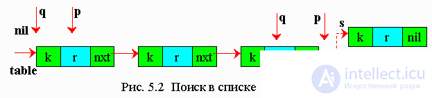
If the data table is specified in the form of a singly linked list, then a sequential search is performed in the list (Fig. 5.2).
Variants of algorithms:
On pseudocode : q = nil p = table while (p <> nil) do if k (p) = key then search = p return endif q = p p = nxt (p) endwhile s = getnode k (s) = key r (s) = rec nxt (s) = nil if q = nil then table = s else nxt (q) = s endif search = s return |
In Pascal : q: = nil; p: = table; while (p <> nil) do begin if p ^ .k = key then begin search = p; exit; end; q: = p; p: = p ^ .nxt; end; New (s); s ^ .k: = key; s ^ .r: = rec; s. ^ nxt: = nil; if q = nil then table = s else q. ^ nxt = s; search: = s; exit |
The advantage of the list structure is the accelerated algorithm for deleting or inserting an element into the list, and the time of insertion or deletion does not depend on the number of elements, and in the array each insertion or deletion requires about half of the elements to move. The effectiveness of the search in the list is about the same as in the array.
Efficiency sequential search can be increased.
Let it be possible to accumulate requests for the day, and at night to process them. When requests are collected, they are sorted.
5.2. Index-sequential searchIn this search, two tables are organized: a data table with its keys (ordered in ascending order) and an index table, which also consists of data keys, but these keys are taken from the main table at a certain interval (Fig. 5.3). First, a sequential search is performed in the index table by the specified search argument. As soon as we pass the key, which turned out to be less than the specified, then we set the lower limit of the search in the main table - low, and then - the upper limit - hi, on which (kind> key). For example, key = 101. The search does not go across the table, but from low to hi.  Examples of programs:
5.3. Sequential Search EfficiencyThe effectiveness of any search can be evaluated by the number of comparisons C of the search argument with the keys of the data table. The smaller the number of comparisons, the more effective the search algorithm. Efficiency of sequential search in an array: C = 1 ¸ n, C = (n + 1) / 2. The effectiveness of a sequential search in the list is the same. Although by the number of comparisons, searching in a linked list has the same efficiency as searching in an array, organizing the data into an array and a list has its advantages and disadvantages. The purpose of the search is to perform the following procedures:
The first procedure (the actual search) takes one time for them. The second and third procedures for the list structure are more efficient (since arrays need to move elements). If k is the number of movements of elements in the array, then k = (n + 1) / 2. 5.4. The effectiveness of index-sequential search
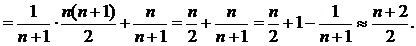
Sequential search Searching for the desired record in an unsorted list is reduced to viewing the entire list before the record is found. "To start from the beginning and continue until the key is found, then stop" [1] is the simplest of the search algorithms. This algorithm is not very efficient, but it works on an arbitrary list. The search algorithm is faced with the important task of determining the location of the key, so it returns the index of the record containing the desired key. If the search failed (no key value was found), then the search algorithm usually returns an index value that exceeds the upper bound of the array. Hereinafter, it is assumed that array A consists of records, and its description and assignment is performed outside the procedure (the array is global with respect to the procedure). The only thing you need to know about the type of records is that the record includes the key field - the key by which the search is performed. Records go sequentially in the array and there are no gaps between them. Record numbers go from 1 to n - the total number of records. This will allow us to return 0 if the target element is not in the list. For simplicity, we assume that key values are not repeated. SequentialSearch Procedure performs a sequential search for the element z in the array A [1 .. n ]. SequentialSearch ( A , z, n) (1) for i ← 1 to n (2) do if z = A [ i ]. key (3) then return i (4) return 0 Worst Case Analysis. The sequential search algorithm has two worst cases. In the first case, the target element is the last in the list. In the second, it is not on the list at all. In both cases, the algorithm will perform n comparisons, where n is the number of elements in the list. Case analysis. The target value may occupy one of n possible positions. We will assume that all these positions are equally probable, i.e., the probability of meeting each of them is
If the target value may not appear in the list, the number of possibilities increases to n + 1. in the absence of an element in the list, its search requires n comparisons. If we assume that all n + 1 possibilities are equally probable, then we obtain
It turns out that the possibility of the absence of an element in the list increases the complexity of the average case by Consider the general case when the probability of meeting the desired item in the list is p i where p i ≥ 0 and
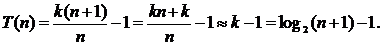
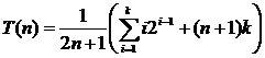
The sequential data retrieval algorithm is equally efficiently performed when placing the set a 1 , a 2 , ..., a n on adjacent or connected memory. The complexity of the algorithm is linear - O ( n ). Logarithmic search Logarithmic (binary or halving) data search is applicable to a sorted set of elements a 1 < a 2 < ... < a n , the placement of which is performed on adjacent memory. The essence of this method is as follows: the search begins with the middle element. When comparing the target value with the middle element of the sorted list, one of three results is possible: the values are equal, the target value is less than the list item, or the target value is larger than the list item. In the first and best case, the search is complete. In the remaining two cases, we can drop half the list. Indeed, when the target value is less than the middle element, we know that if it is in the list, it is before this middle element. If the target value is greater than the middle element, we know that if it is in the list, then it is after this middle element. This is enough for us to drop half the list with one comparison. So, the comparison result allows you to determine in which half of the list to continue the search, applying the same procedure to it. BinarySearch Procedure performs a binary search for the element z in a sorted array A [1 .. n ]. BinarySearch (A, z , n ) (1) p ← 1 (2) r ← n (3) while p ≤ r do (4) q ← [( p + r ) / 2] (5) if A [ q ]. key = z (6) then return q (7) else if A [ q ]. key < z (8) then p ← q +1 (9) else r ← q -1 (10) return 0 Worst Case Analysis . Since the algorithm divides the list in half each time, we will assume in the analysis that n = 2 k - 1 for some k . It is clear that on some passage the cycle deals with a list of 2 j - 1 items. The last iteration of the loop is performed when the size of the remaining part becomes equal to 1, and this happens when j = 1 (since 2 1 - 1 = 1). This means that for n = 2 k - 1 the number of passes does not exceed k . Therefore, in the worst case, the number of passes is k = log 2 ( n + 1). Case analysis . We consider two cases. In the first case, the target value is probably contained in the list, and in the second it may not be there. In the first case, the target value n possible provisions. We assume that they are all equally probable. Imagine the data a 1 < a 2 < ... < a n in the form of a binary comparison tree that corresponds to a binary search. A binary tree is called a comparison tree if the condition is satisfied for any of its vertices: {Tops of the left subtree} <{Top of the root} <{Tops of the right subtree} If we consider the binary comparison tree, then for elements at nodes of level i i required comparisons. Since at level i there are 2 i ‑ 1 nodes, and for n = 2 k - 1 in the tree of k levels, the total number of comparisons for all possible cases can be calculated by summing the product of the number of nodes at each level by the number of comparisons at this level.
Substituting 2 k = n + 1, we obtain
In the second case, the number of possible positions of the element in the list is still n , but this time there are n + 1 possibilities for the target value not from the list. The number of possibilities is n + 1, since the target value can be less than the first element in the list, more than the first, but less than the second, more than the second, but less than the third, and so on, up to the possibility that the target value is more than the nth element. In each of these cases, the absence of an element in the list is detected after k comparisons. In total, 2 n + 1 possibilities are involved in the calculation.
Similarly, we obtain
Hence, the complexity of the search is logarithmic O (log 2 n ). The considered binary search method is mainly intended for sorted elements a 1 < a 2 < ... < a n on adjacent memory of a fixed size. If the dimension of the vector changes dynamically, then the savings from the use of binary search will not cover the costs of maintaining an ordered arrangement a 1 < a 2 < ... < a n .
Overview of Search Algorithms and Methods
Graph Search Algorithms Combinatorial optimization Substring search Apriori Algorithm |

 +1
+1 )
) . Therefore, to find the ith element of A [ i ], i comparisons. As a result, for complexity in the average case, we obtain the equality
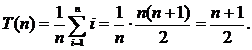
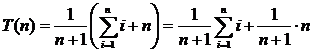
 , but compared with the length of the list, which can be very long, this value is negligible.
 In this case, the average complexity (mathematical expectation) of the element search will be equal to
  A good approximation of the frequency distribution to reality is Zipf's law:
  for i = 1, 2, ..., n . [ n is the most commonly used word in a natural language text with a frequency approximately inversely proportional to n .] The normalizing constant is chosen so that
 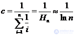 and the average time for a successful search will be
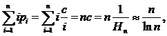 which is much less
  . This suggests that even a simple sequential search requires the selection of a reasonable set data structure that would increase the efficiency of the algorithm.

 .
.

Comments
To leave a comment
Structures and data processing algorithms.
Terms: Structures and data processing algorithms.