Addressing Elements Using Iliffe Vectors

Recall the basic concepts of arrays

1 Array as a logical structure

2. Array as a physical structure

3. Array operations

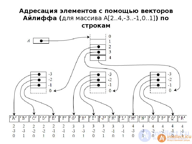
4. Addressing elements using Iliffe vectors

5 Examples of representing arrays using Iliffe vectors

In computer programming, an Iliffe vector, also known as a display, is a data structure used to implement multi-dimensional arrays. An Iliffe vector for an n-dimensional array (where n ≥ 2) consists of a vector (or 1-dimensional array) of pointers to an (n − 1)-dimensional array. They are often used to avoid the need for expensive multiplication operations when performing address calculation on an array element. They can also be used to implement jagged arrays, such as triangular arrays, triangular matrices and other kinds of irregularly shaped arrays. The data structure is named after John K. Iliffe.

Born 18 September 1931 London

1 Array as a logical structure

An array is such a data structure that is characterized by:

• a fixed set of elements of the same type;
• each element has a unique set of index values;
• the number of indices determines the dimension of the array, for example, two indices - a two-dimensional array, three indices - a three-dimensional array, one index - a one-dimensional array or vector;
• access to an array element is performed by the name of the array and index values ​​for this element.

Another definition: an array is a vector, each element of which is a vector.

The syntax for describing the array is represented as:

      : Array [n1..k1] [n2..k2] .. [nn..kn] of . 

For the case of a two-dimensional array:

       Mas2D: Array [n1..k1] [n2..k2] of , or
       Mas2D: Array [n1..k1, n2..k2] of  

Visual two-dimensional array can be represented in the form of a table of (k1-n1 + 1) rows and (k2-n2 + 1) columns.

2. Array as a physical structure

The physical structure is the placement of array elements in computer memory. For the case of a two-dimensional array consisting of (k1-n1 + 1) rows and (k2-n2 + 1) columns, the physical structure is shown in Fig. 3.3.

Fig. 3.3. Physical structure of a two-dimensional array of (k1-n1 + 1) rows and (k2-n2 + 1) columns

Multidimensional arrays are stored in contiguous memory. The slot size is determined by the base type of the array element. The number of array elements and the size of the slot determine the size of the memory for storing the array. The principle of distribution of array elements in memory is determined by the programming language. So in FORTRAN the elements are distributed in columns - so that the left indexes change faster, in PASCAL - in rows - the index changes in the direction from right to left.

The number of memory bytes occupied by a two-dimensional array is determined by the formula:

   ByteSize = (k1-n1 + 1) * (k2-n2 + 1) * SizeOf (Type) 

The address of the array is the address of the first byte of the initial component of the array. The offset to the array element Mas [i1, i2] is determined by the formula:

         ByteNumber = [(i1-n1) * (k2-n2 + 1) + (i2-n2)] * SizeOf (Type)
 his address is @ByteNumber = @mas + ByteNumber.
      For example:
      var Mas: Array [3..5] [7..8] of Word; 

The basic type of the Word element requires two bytes of memory, then the table 3.2 of the offset of the array elements relative to @Mas will be as follows:

Table 3.2

This array will occupy in memory: (5-3 + 1) * (8-7 + 1) * 2 = 12 bytes; and the address of the element Mas [4.8]:

    @Mas + ((4-3) * (8-7 + 1) + (8-7) * 2 = @ Mas + 6 

3. Array operations

The most important physical layer operation on an array is access to a given element. As soon as access to an element is implemented, any operation that makes sense for the data type to which the element corresponds can be performed on it. The transformation of a logical structure into a physical one is called a linearization process, during which the multidimensional logical structure of the array is transformed into a one-dimensional physical structure.

In accordance with formulas (3.3), (3.4) and by analogy with the vector (3.1), (3.2) for a two-dimensional array with the boundaries of the indices:

[B (1) .. E (1)] [B (2) .. E (2)] located in the memory in rows, the address of the element with indices [I (1), I (2)] can be calculated as :

  Addr [I (1), I (2)] = Addr [B (1), B (2)] +
  {[I (1) -B (1)] * [E (2) -B (2) +1] + [I (2) -B (2)]} * SizeOf (Type) (3.5)
      Generalizing (3.5) for an array of arbitrary dimension:
            Mas [B (1) .. E (2)] [B (2) .. E (2)] ... [B (n) .. E (n)]
 we get:
      Addr [I (1), I (2), ..., I (n)] = Addr [B (1), B (2), ... B (n)] -
                 nn (3.6)
 - Sizeof (Type) * AMOUNT [B (m) * D (m)] + Sizeof (Type) * AMOUNT [I (m) * D (m)]
                m = 1 m = 1 

where Dm depends on how the array is placed. When placing in rows:

      D (m) = [E (m + 1) -B (m + 1) +1] * D (m + 1), where m = n-1, ..., 1 and D (n) = 1 

when placed in columns:

      D (m) = [E (m-1) -B (m-1) +1] * D (m-1), where m = 2, ..., n and D (1) = 1 

When calculating the address of an element, the most difficult is the calculation of the third component of formula (3.6), because the first two are independent of indices and can be calculated in advance. To speed up the calculations, the factors D (m) can also be calculated in advance and stored in an array descriptor. The array descriptor thus contains:

• the starting address of the array is Addr [I (1), I (2), ..., I (n)];
• the number of measurements in the array is n;
• the constant component of the linearization formula (the first two components of formula (3.6);
• for each of n dimensions of the array:
  • boundary index values ​​- B (i), E (i);
  • the linearization formula factor is D (i).

One of the definitions of an array is that it is a vector, each element of which is a vector. Some programming languages ​​allow you to select one or more dimensions from a multidimensional array and consider them as an array of lower dimensionality.

For example, if a two-dimensional array is declared in a PL / 1 program:

                  DECLARE A (10.10) BINARY FIXED; 

then the expression: A [*, I] - will refer to a one-dimensional array consisting of elements: A (1, I), A (2, I), ..., A (10, I).

The joker symbol "*" means that all elements of the array are selected according to the dimension to which the index specified by the joker corresponds. Using the joker also allows you to set group operations on all elements of the array or on its selected dimension,

                  for example: A (*, I) = A (*, I) + 1 

The operations of the logical level on arrays should include such as sorting an array, searching for an element by key. The most common search and sorting algorithms will be discussed in this chapter below.

4. Addressing elements using Iliffe vectors

It can be seen from the above formulas that calculating the address of an element of a multidimensional array can take a lot of time, since addition and multiplication operations must be performed, the number of which is proportional to the dimension of the array. The operation of multiplication can be excluded by applying the following method.

Fig. 3.4. Representation of arrays using Isliff vectors

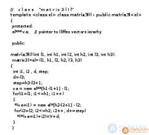
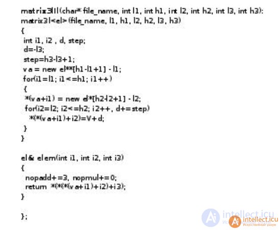
For an array of any dimension, a set of descriptors is formed: the main and several levels of auxiliary descriptors called Ailiff vectors. Each Ailiff vector of a certain level contains a pointer to the zero components of the Ailiff vectors of the next, lower level, and the Ailiff vectors of the lowest level contain pointers to groups of elements of the displayed array. The main array descriptor stores the first level Isliff vector pointer. With such an organization, an arbitrary element B (j1, j2, ..., jn) of a multidimensional array can be accessed by going through the chain from the main descriptor through the corresponding components of the Ayliffe vectors.

In fig. 3.4 shows the physical structure of the three-dimensional array B [4..5, -1..1,0..1], presented by the method of Isliff. It can be seen from this figure that the Ayliff method, increasing the speed of access to the array elements, at the same time leads to an increase in the total memory required for representing the array. This is the main drawback of representing arrays using Ailiff vectors.

5 Examples of representing arrays using Iliffe vectors