Lecture
| Data structures (list) | |
|---|---|
| Types |
Collection • Container |
| Arrays |
Associative array • Multimap • Set • Multiset • Hash table |
| Lists |
Linked list • Queue (Ring buffer • Biconnected) • Stack • List with gaps |
| Trees |
B-tree • Binary search tree • Heap |
| Counts |
Oriented graph • Directed acyclic graph • Binary diagram of solutions • Hypergraph |
A necessary condition for storing information in computer memory is the ability to convert this very information into a suitable form for a computer. In the event that this condition is fulfilled, it is necessary to determine the structure suitable for the available information, the one that will provide the required set of opportunities to work with it. Here, a structure is understood as a way of presenting information, by means of which a set of separately taken elements forms something united, due to their interconnection with each other. Arranged according to some rules and logically interconnected, the data can be processed very efficiently, since the common structure provides them with a set of management capabilities — one of which means that high results are achieved in solving various tasks. But not every object is represented in an arbitrary form, and perhaps there is only one single method of interpretation for it, therefore, the undoubted advantage for the programmer will be the knowledge of all existing data structures. Thus, it is often necessary to make a choice between different methods of storing information, and the performance of a product depends on such a choice.
Speaking of non-computing, you can show no case where the information is visible structure. A good example is the book of a very different content. They are divided into pages, paragraphs and chapters, they usually have a table of contents, that is, an interface for using them. In a broad sense, every living being has a structure; without it, organics could hardly exist.
It is likely that the reader had to deal with data structures directly in computer science, for example, those that are built into the programming language. Often they are referred to as data types. These include: arrays, numbers, strings, files, etc.
Methods of storing information, called "simple", i.e. indivisible into component parts, are preferable to study with a specific programming language, or to go deeply into the essence of their work. Therefore, only “integrated” structures will be considered here, those that consist of simple structures, namely: arrays, lists, trees and graphs.
An array is a data structure with a fixed and ordered set of similar elements (components). Access to any of the elements of the array is carried out by name and number (index) of this element. The number of indices determines the dimension of the array. For example, one-dimensional (vectors) and two-dimensional (matrices) arrays are most common. The first have one index, the second - two. Let a one-dimensional array be called A, then in order to gain access to its i-th element, you need to specify the name of the array and the number of the required element: A [i]. When A is a matrix, it is represented in the form of a table, the elements of which are accessed by the array name, as well as the row and column numbers, at the intersection of which the element is located: A [i, j], where i is the row number, j is the number column
In different programming languages, working with arrays may differ somewhat, but the basic principles are usually the same everywhere. In the Pascal language, reference to a one-dimensional and two-dimensional array occurs exactly as shown above, and, for example, in C ++, the two-dimensional array should be specified as follows: A [i] [j]. The array elements are numbered alternately. The meaning of the numbering is influenced by the programming language. Most often this value is 0 or 1.
Arrays of the type described are called static, but there are also arrays for certain characteristics that are different from them: dynamic and heterogeneous. The dynamism of the former is characterized by inconsistency in size, that is, as the program runs, the size of the dynamic array may change. This function makes working with data more flexible, but at the same time you have to sacrifice speed, and the process itself becomes more complicated. A mandatory criterion for a static array, as has been said, is the homogeneity of the data stored simultaneously in it. When this condition is not met, the array is heterogeneous. Its use is due to shortcomings that are in the previous form, but it is justified in many cases.
Thus, even if you have decided on a structure, and have chosen an array as its structure, this is still not enough. After all, an array is just a general designation, a genus for a number of possible implementations. Therefore, it is necessary to decide on a specific presentation method, with the most appropriate array.
A list is an abstract data type that implements an ordered set of values. Lists differ from arrays in that access to their elements is performed sequentially, while arrays are a random access data structure. This abstract type has several implementations in the form of data structures. Some of them will be reviewed here.
A list (linked list) is a data structure that represents a finite set of ordered elements connected with each other by means of pointers. Each structure element contains a field with some information, as well as a pointer to the next element. Unlike an array, there is no random access to the elements of the list.
Singly linked list
In the simply linked list given above, the starting element is the Head list (the list head [arbitrary name]), and everything else is called the tail. The tail of the list consists of elements divided into two parts: informational (info field) and index (next field). In the last element, instead of the pointer, the end of the list attribute is nil.
A simply-connected list is not very convenient, since from one point it is possible to get only to the next point, thus moving to the end. When, in addition to the pointer to the next element, there is a pointer to the previous one, such a list is called doubly linked.
Doubly linked list
The ability to move both forward and backward is useful for some operations, but additional pointers require more memory than is needed in an equivalent, simply linked list.
For the two kinds of lists described above, there is a subspecies called the ring list. You can make a ring from a single-connected list by adding just one pointer to the last element, so that it refers to the first one. And for a doubly-connected one, two pointers are required: the first and the last elements
Ring List
In addition to the considered types of list structures, there are other ways of organizing data by the “list” type, but they, as a rule, are very similar to the parsed ones, so they will be omitted here.
In addition to the differences in relationships, the lists are divided according to the methods of working with data. Some of these methods are described below.
Stack
The stack is characterized by the fact that it can only be accessed from one end, called the top of the stack, in other words: the stack is a data structure that functions according to the LIFO principle (last in - first out, “last came - first out”). It is better to depict this data structure in the form of a vertical list, for example, piles of some things, where in order to use one of them you need to pick up all those things that lie above it, and you can put the object only on the top of the stack.
In the single-linked list shown, operations on elements occur strictly at one end: to include the desired element in the fifth cell, it is necessary to exclude the element that occupies this position. If there were, for example, 6 elements, and it was also necessary to insert a specific element in the fifth cell, then we would have to exclude two elements.
The “Queue” data structure uses the FIFO organization principle (First In, First Out - “first in, first out”). In a sense, this method is fairer than the one on which the stack functions, because the simple rule underlying the usual queues at various stores, hospitals is considered to be quite fair, and it is the basis of this structure. Let this observation be an example. Strictly speaking, a queue is a list, adding elements to which is permissible only at its end, and their extraction is done from the other side, called the beginning of the list.
Turn
This structure simultaneously operates in two ways to organize data: FIFO and LIFO. Therefore, it is permissible to attribute it to a separate program unit, resulting from the summation of the two previous types of list.
Dec (deque - double ended queue, “double-sided queue”) - stack with two ends. Indeed, despite a specific translation, decks can be defined not only as a two-way queue, but also as a stack that has two ends. This means that this kind of list allows you to add elements to the beginning and to the end, and the same is true for the extraction operation.
Dec
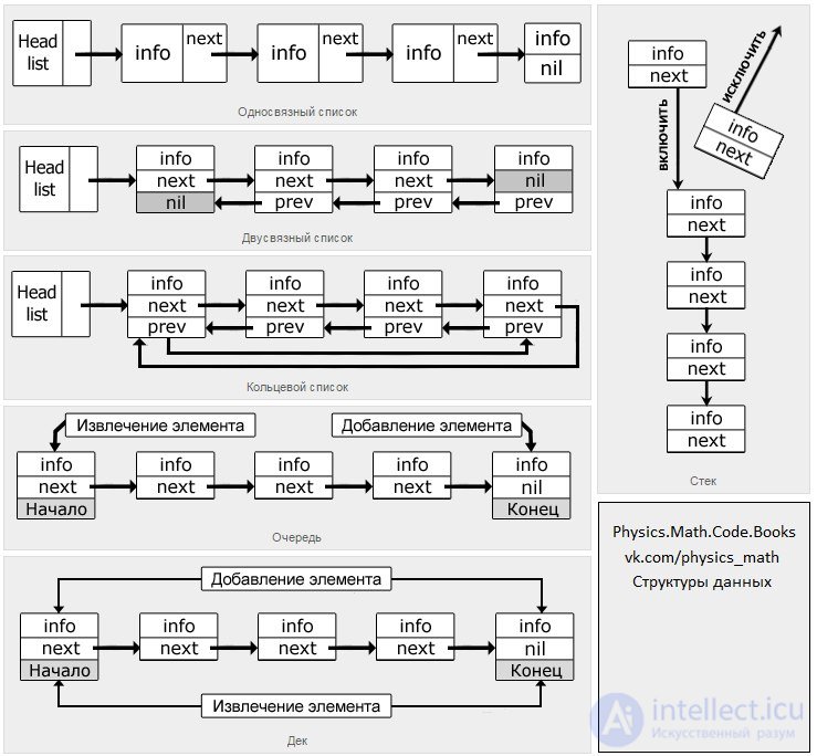
This structure simultaneously works in two ways to organize data: FIFO and LIFO. Therefore, it is permissible to attribute it to a separate program unit, resulting from the summation of the two previous types of list.
The section of discrete mathematics that studies graphs is called graph theory. In graph theory, well-known concepts, properties, methods of representation, and areas of application of these mathematical objects are considered in detail. We are interested in only those aspects of it that are important in programming.
A graph is a collection of points connected by lines. Points are called vertices (nodes), and lines - edges (arcs).
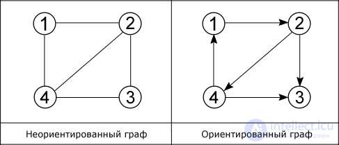
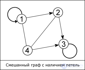
As shown in the figure, there are two main types of graphs: oriented and non-oriented. In the first edges are directed, that is, there is only one available direction between two connected vertices, for example, from vertex 1 you can pass to vertex 2, but not vice versa. In an undirected connected graph from each vertex you can go to each and back. A special case of these two types is a mixed graph. It is characterized by the presence of both oriented and non-oriented edges.
The degree of entry of a vertex is the number of edges included in it, the degree of exit is the number of outgoing edges.
The edges of the graph do not have to be straight, and the vertices are denoted by numbers, as shown in the figure. In addition, there are such graphs, the edges of which are assigned to a specific value, they are called weighted graphs, and this value - the weight of the edge. When both ends of the edge coincide, that is, the edge goes out from the vertex F and enters it, then this edge is called a loop.
Graphs are widely used in structures created by man, for example, in computer and transport networks, web-technologies. Special presentation methods allow the use of a graph in computer science (in computers). The most famous of them are: “The matrix of contiguity”, “The matrix of incidence”, “List of contiguity”, “List of ribs”. The first two, as the name implies, use a matrix to represent the graph, and the last two use a list.
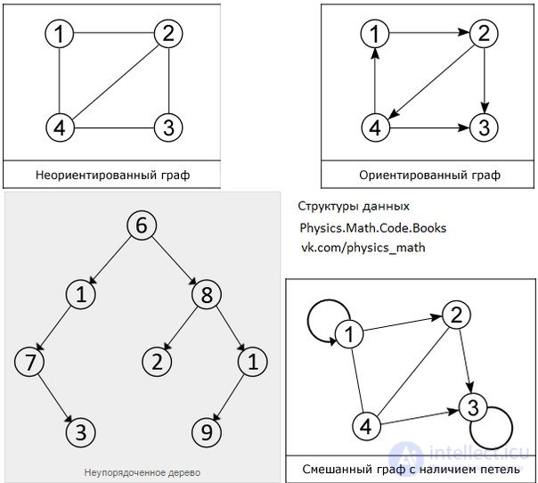
Disordered tree
A tree as a mathematical object is an abstraction of co-occurring units found in nature. The similarity of the structure of natural trees with graphs of a certain type indicates the assumption of establishing an analogy between them. Namely, with connected and with it acyclic (not having cycles) graphs. The latter in their structure really resemble trees, but there are some differences, for example, it is customary to depict mathematical trees with the root located at the top, i.e., all branches “grow” from top to bottom. It is known that in nature it is not so at all.
Since a tree is inherently a graph, many of its definitions coincide with the latter, or they are intuitively similar. So the root node (vertex 6) in the tree structure is the only vertex (node), characterized by the absence of ancestors, i.e. such that no other vertex refers to it, and from the root node itself you can reach any of the existing vertices tree, which follows from the connectivity property of this structure. Nodes that do not refer to any other nodes, in other words, those with no descendants are called leaves (2, 3, 9) or terminal nodes. The elements located between the root node and the leaves are intermediate nodes (1, 1, 7, 8). Each tree node has only one ancestor, or if it is the root, it does not have one.
A subtree is a part of a tree that includes some root node and all its descendant nodes. For example, in the figure, one of the subtrees includes root 8 and elements 2, 1, 9.
You can perform many operations with a tree, for example, find elements, delete elements and subtrees, insert subtrees, find root nodes for some vertices, etc. One of the most important operations is tree traversal. There are several workarounds. The most popular of them: symmetric, direct and reverse bypass. During the forward walk, the ancestor nodes are visited before their descendants, and in the reverse round, the opposite situation is respectively. In symmetric traversal, the subtrees of the main tree are alternately viewed.
Presentation of data in the considered structure is beneficial if the information has an explicit hierarchy. For example, working with data on biological genera and species, official positions, geographic features, etc., requires a hierarchically expressed structure, such as mathematical trees.

Comments
To leave a comment
Structures and data processing algorithms.
Terms: Structures and data processing algorithms.