Lecture
In a special type of graphs, trees are highlighted. A tree is a connected graph that does not have cycles, since any two of its vertices are connected in a simple way. In fig. Figure 4.14 shows all five tree species that can be obtained at six vertices.
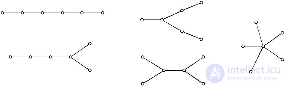
Fig. 4.14
An oriented tree is an infinite digraph, in which a negative semi-degree ρ is any vertex no more than 1 and there is exactly one vertex, called the root of an oriented tree, with a negative degree ρ– = 0.
Based on this definition, one can prove that in a oriented tree any vertex is reachable from the root. The main properties of trees are described by the following theorem.
Theorem 4.3
1. In an undirected tree, there are at least two terminal vertices.
2. Between any two vertices of the tree there is exactly one path.
3. The number of edges in the tree is always one less than the number of vertices ( m = n –1 ).
Since all paths in a tree are simple, there is at least one maximum path in it, that is, a path that cannot be continued. The ends of this path are the terminal vertices.
The presence of a path between any pair of vertices follows from the connectedness of the tree, and the uniqueness of this path from the fact that the existence of two paths between a pair of vertices always creates a cycle.
The third point of the theorem is easiest to prove using the concept of an oriented tree. Select an arbitrary vertex in the tree. Let's call it a root. Edges incident to the root, oriented in the direction from the root. For each vertex v i that is the end of one of these edges, we orient the remaining edges to it from v i . We continue this procedure until the end vertices are reached. Due to the uniqueness of the path between the vertices, no vertex will be reached twice (that is, it will not be necessary to orient already oriented edges), and by virtue of the connectedness of the tree all vertices will be reached. From this procedure, it is clear that the root has no incoming edges, and all other vertices have one incoming edge. Since all edges are incoming for some vertex and in the process of orientation the number of vertices and edges has not changed, then Section 3 of the theorem follows from this.
For oriented trees, properties 1 and 3 are always true, but property 2 is not. That is why an oriented tree: 1) is always weakly connected; 2) is one-sidedly connected only if it is an oriented chain (that is, when all the vertices lie on a unique path from the root); 3) is never strongly connected, since a strongly connected graph necessarily contains a cycle.
For all vertices of an oriented tree, with the exception of the root, negative semi-degree ρ– = 1, and positive semi-degree ρ + can take any value from zero. Moreover, those vertices with positive semi-degree ρ + = 0 are called tree leaves . An oriented tree, in which each vertex, distinct from the root, has a leaf, is called a bush .
Consider some parameters that characterize an oriented tree.
 v 0 Level 3
v 1 v 2 v 3 Level 2
v 4 v 5 v 6 v 7 v 8 Level 1
v 9 Level 0
Fig. 4.15
The height of the oriented tree is the longest path length from root to leaf; the depth of the vertex of the oriented tree is the length of the path from the root to this vertex; vertex height is the longest path length from a given vertex to a leaf, and finally, the vertex level of an oriented tree is the difference between the height of the oriented tree and the depth of the vertex. From these definitions, we can conclude that the root level is equal to the height of the tree, but the levels of different leaves, like their depths, can be different, but the height of any leaf is zero (Fig. 4.15).
When identifying trees, the root form of the tree view is convenient. When choosing a root from a tree, all terminal vertices and edges are successively removed until one or two vertices remain. In the first case, the remaining vertex is selected as the root and is called the center. In the second case, the vertices and the edge connecting them form a bicenter .
In another method of selecting the root of a tree, the concept of the height of the top is used. Each vertex has branches that are parts of the tree. The vertex with the smallest height is chosen as the root and is called the centroid . If there are two such vertices, then they, together with the edge that unites them, form a centroid . In this case, the vertex is taken as the root from which a tree grows with a smaller number of vertices.
Any boolean function can be visualized as an oriented tree. Moreover, the leaves of this tree are labeled with variables or constants of a logical equation, and each node that is not a leaf is marked with one of the operations of Boolean algebra. An example of such a tree for the function

shown in fig. 4.16
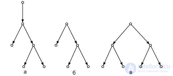
ABOUT 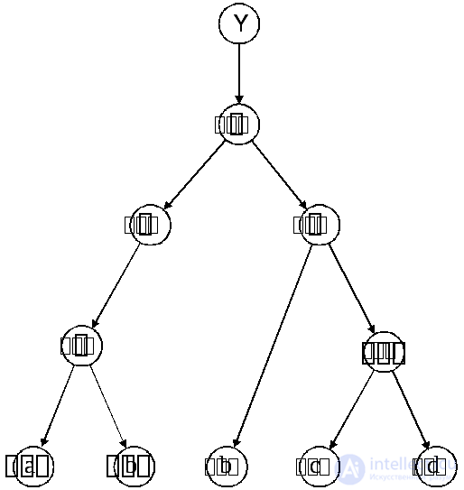 A oriented tree is called binary if the positive semi-degree of any of its vertices is not greater than 2; A binary oriented tree is called complete if exactly two arcs emanate from any of its vertices that are not a leaf, and the leaf levels coincide. Examples of various binary oriented trees are shown in Fig. 4.17. In fig. 4.17a, b shows incomplete oriented binary trees, in fig. 4.17v - complete. Fig. 4.16
Theorem 4.4 (theorem on the height of a binary oriented tree with a given number of leaves). Binary oriented tree with n leaves has a height not lower than log 2 n .
This theorem has one very interesting application. Suppose that it is necessary to arrange strictly ascending the elements of the finite linearly ordered set { a 1 , ..., a n }. This task is called a sorting task, and any algorithm that solves it is called a sorting algorithm. From a mathematical point of view, the sorting algorithm should find such a permutation { a i 1 ,. . . , and i n } of the elements of the set that would be consistent with the relation ≤ linear order given on it, i.e. for any k , l from the validity of the inequality i k < i l must follow a ik ≤ a il
 v 0
v 0
v 1 v 0 v 0
v 2 v 3 v 1 v 2 v 1 v 2
v 4 v 5 v 3 v 4 v 3 v 4 v 5 v 6
Fig. 4.17
Initially sorted elements can be arranged in any order, i.e. Any permutation of the elements of a sortable set can be original, and we have no a priori information about this permutation. The only way to obtain such information is to make pairwise comparisons of the elements a i , (relative to the linear order under consideration) in any sequence. Note that it is not necessary to make all possible comparisons, i.e. compare a i with a j for all i ≠ j . For example, you can use the transitivity of an order relation.
All comparisons, which in principle can be made in the process of working of some algorithm, are visualized in the form of an oriented tree, called a decision tree . In fig. Figure 4.18 shows the decision tree for the three-element set { a, b , c }. The vertices of the oriented tree that are not leaves are labeled with the checked inequalities, and the set of leaves is in one-to-one correspondence with the set of all permutations of the original set.
Since the sorting can result in any permutation of the original set and each such permutation corresponds to a leaf of the decision tree, in the general case the number of leaves will be equal to n ! - the number of permutations of the n- element set.
Therefore, sorting the input sequence, the algorithm will necessarily go some way from the root of the decision tree to one of the leaves and, thus, the number of comparison operations (the number of steps of the sorting algorithm) will be proportional to the height of the decision tree, not less than log 2 n ! , by virtue of Theorem 4.4. Using the Stirling formula for evaluating factorial for large n
 ,
,
we obtain that the decision tree has a height of order n log 2 n .
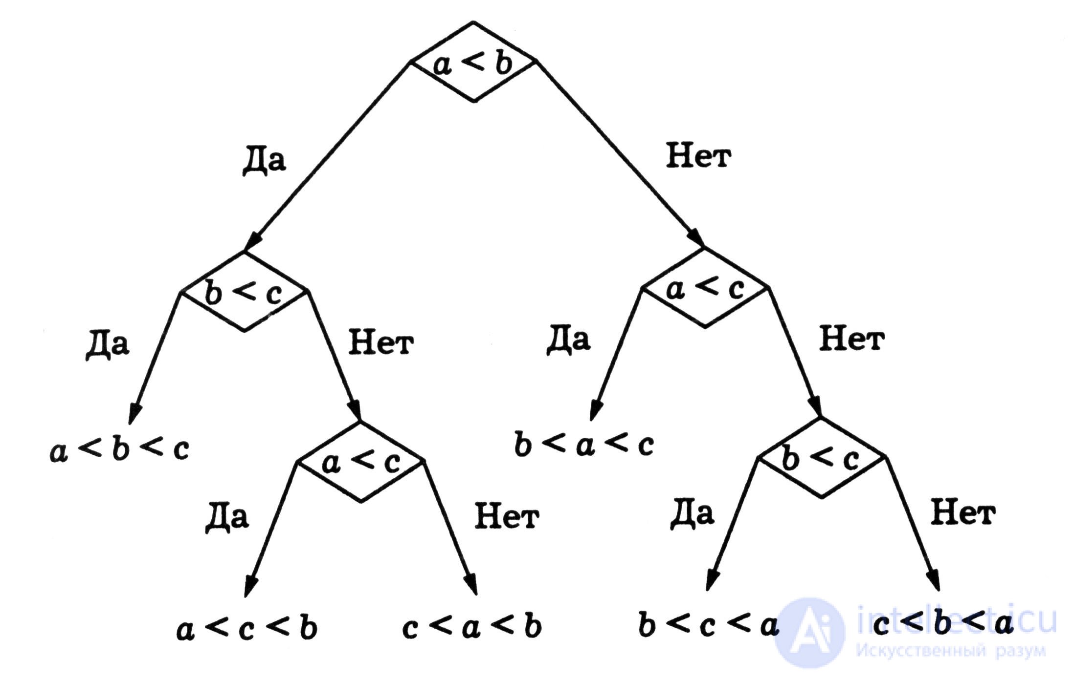
Fig. 4.18
Thus, in the general case, the problem of sorting using pairwise comparisons cannot be solved faster than in a specified number of steps. Of course, the specific path in the decision tree from the root to one of the leaves depends on the original permutation. For example, in the decision tree shown in fig. 4.18, there are two “short” paths of length 2, but the remaining paths are of length 3.
Note that, in the general case, an oriented tree is not a connected oriented graph. The components of the oriented tree are its subgraphs generated by a set of vertices located on some path from root to leaf.
In conclusion of this chapter, it should be noted once again that graphs are one of the most common languages for representing various mathematical objects and formulating various theoretical and applied problems that go beyond the limits of graph theory itself. It is difficult to name an application area where graph theory is not applied. Graphs are used in mathematical logic and the theory of formal systems, in the theory of algorithms and theoretical programming (for the representation and analysis of algorithms and programs), in the theory of languages and grammars (for syntactic analysis of texts). They are used to describe and analyze both static structures (organizational structures, transport networks) and dynamic systems in which the vertices correspond to the state of the system, and oriented edges correspond to transitions from one state to another. It is graphs that are the most convenient means of formalized representation of finite automata.
Control tasks
1. How many undirected graphs with n vertices exist?
2. Prove that the sum of the degrees of all vertices of an undirected graph is equal to twice the number of edges (this statement is known as the “handshake lemmas”).
3. Establish which of the images shown in fig. 4.19 graphs are isomorphic and which are not.
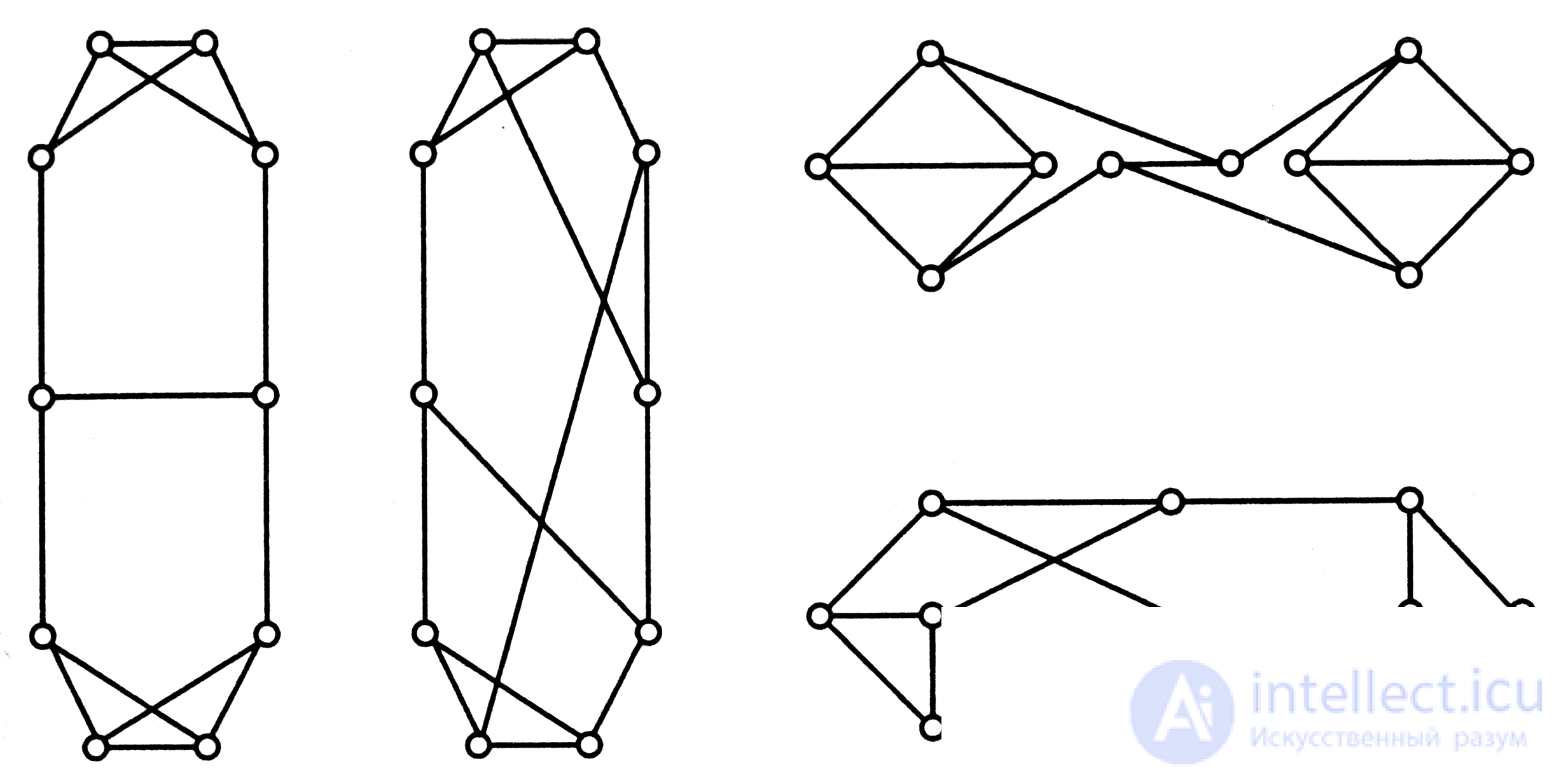
Fig. 4.19
four 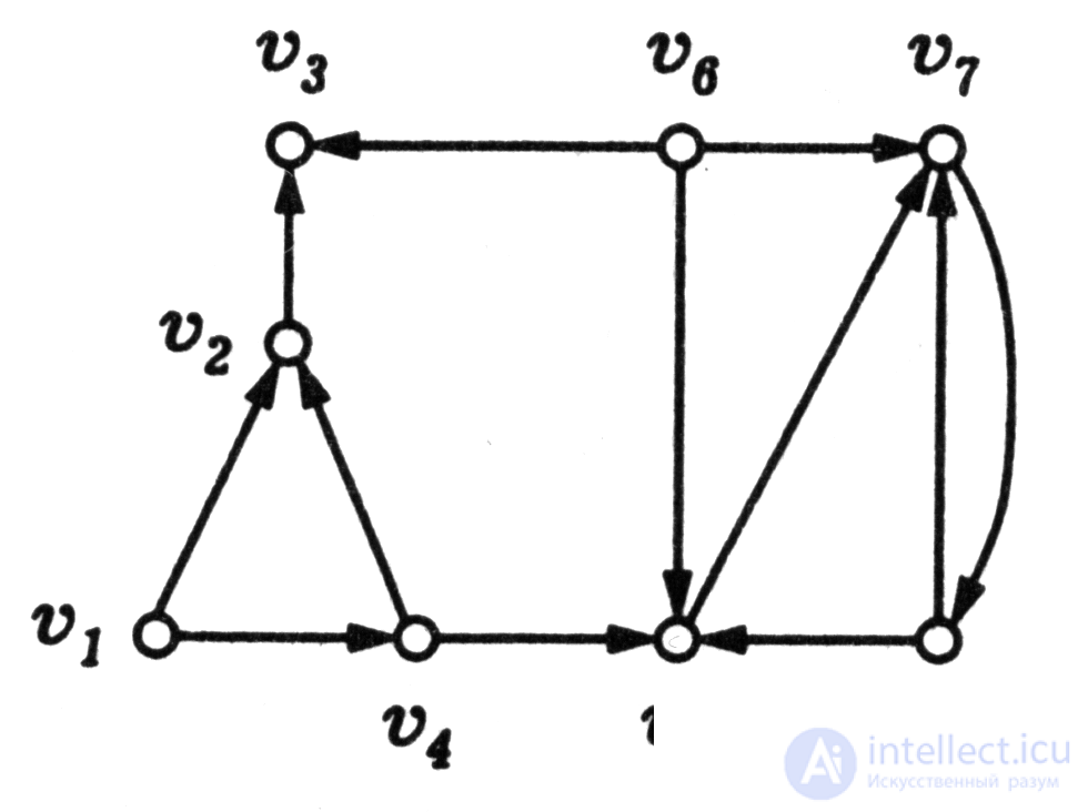 . Find all pairwise nonisomorphic graphs undirected graphs with four vertices and three edges.
5. Determine whether the directed graph shown in Fig. 4.20, connected. Build an adjacency matrix for this graph.
6. Prove that a connected undirected graph has an Euler cycle if and only if the degree of each of its vertices is even. Fig. 4. 20
7. The incidentor of the graph P is determined by the values: P (a, 1, b); P (b, 2, b); P (b, 3, s); P (e, 4, b); P (c, 5, d); P (d, 6, s); P (f, 7, c); P (d, 8, d); P (e, 9, d); P (a, 10, e); P (a, 11, d); P (a, 12, f) - which are true, the rest are false. Build a graph, create a table of adjacency and incidence, determine the center of the graph.
8. The oriented graph is given by the adjacency matrix containing the labels of the corresponding edges: construct a graph and solve the shortest path problem.
 0 7 8 9 10
0 0 8 9 10
0 -2 0 9 10
0 -4 -3 0 10
0 -7 -6 -5 0
9. Prove that a directed graph is connected if and only if it has a path that passes through all vertices. Will this statement be true if we demand that there is a simple way?
10. Calculate the number of trees on the set of p vertices for p = 5, 10, 15, 20. How much time would it take to count trees with a capacity of 106 operations / s, counting one operation per tree?
11. Show that for trees on p tops with p < 5 the centers and centroids (or bicenters and bicentroids) are the same.

Comments
To leave a comment
Finite state machine theory
Terms: Finite state machine theory