5.4. Equivalence of finite automata: Moore's theorem

Two Boolean functions F1 and F2 are equivalent if they take the same values ​​on all possible sets of input variables. Since the number of sets of Boolean functions is finite, then, having gone through all of them, one can check whether F1 and F2 are equivalent. You can also bring F1 and F2 to perfect normal form and compare their representations.

The situation is different with finite automata. Two finite automata are equivalent if the input-output mappings they implement are equivalent. The state machine realizes the mapping of an infinite set of input signal sequences into an infinite set of output signal sequences. Therefore, automaton mappings cannot be compared by simply listing their values ​​on all possible arguments.

The state machines A = {XA, YА, QА, δА, λА} and B = {XВ, YВ, QВ, δВ, λВ} are called equivalent if two conditions are fulfilled:

a) their input alphabets are the same: XA = XB = X;

b) the automaton maps realized by them coincide:

( χХ *) λА * ( q А , χ) = λВ * ( q В , χ).

Equivalence of automata means that any automaton mapping realized by one of them can be realized by another; in other words, their possibilities for implementing the conversion of input information into output information coincide. It is rather difficult to determine the equivalence of two automata by enumerating their reactions on all input words, since there are infinitely many input words. However, there is a fairly simple method for solving this problem, based on the concept of the direct product of automata.

The direct product of finite automata A = {X, YА, QА, δА, λА} and B = {X, YВ, QВ, δВ, λВ} with the same input alphabet X is called А А В В = {X, YА × YВ, QА × QВ, δА × В, λА × В}, where:

but) ( q A  QA) ( q Q  QB) ( x X) δA × B (( q A , q B ) x ) = (δA ( q A , x ), δB ( q B , x ));

b) ( q A  QA) ( q Q  QB) ( x X) λA × B (( q A , q B ) x ) = (λА ( q А , x ), λВ ( q В , x )).

AND 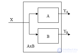First of all, a finite state machine, which is a direct product of two finite automata, has the states of the original automata as its states, the output alphabet is a set of pairs of output symbols of the automata multipliers, and the functions of the outputs and transitions are defined componentwise. Thus, these are just two noninteracting finite automata standing side by side, synchronously operating on one common input (Fig. 5.7). The direct product of automata is also called a synchronous composition. Figure. 5.7

Theorem 5.1. (Theorem Moore) Two finite state machines A = {X, YА, QА, δА, λА} and B = {X, YВ, QВ, δВ, λВ} with the same input alphabet X are equivalent if and only if states ( q A , q B ) in their direct product A × B holds true ( x X) λA ( q A , x ) = = λB ( q B , x ).

Definition: The state q Q is called reachable if and only if ( χХ *) δ * ( q 0 , χ) = q (that is, by the action of any input word χ, the automaton falls into this state.

Evidence. Let A and B are equivalent, that is, by definition, equivalence ( χХ *) λА * ( q А , χ) = λВ * ( q В , χ).

We prove with this assumption:

( ( q A , q B )  QA × QB) is achievable ( q A , q B ) ( x X) λA ( q A , x ) = λB ( q B , x ).

In accordance with the definition, the property of accessibility of a state ( q A , q B ) is equivalent to the condition ( χХ *) δ * (( q 0А , q 0В ) , χ) = ( q А , q В ). Thus, it is necessary to prove that if

( χХ *) λ * ( q 0А , χ) = λ * ( q 0B , χ) then

( ( q A , q B )  QA × QВ) [( ξХ *) δ * (( q 0А , q 0В ) , ξ) = ( q A , q B ) 

 ( x X) λA ( q A , x ) = λB ( q B , x )].

Suppose the contrary, that is what

¬ ( ( q A , q B )  QA × QВ) [( ξХ *) δ * (( q 0А , q 0В ) , ξ) = ( q A , q B ) 

 ( x X) λA ( q A , x ) = λB ( q B , x )], (here, the sign ¬ before the expression defines inversion) and show that then ¬ ( χХ *) λА * ( q 0А , x ) = λВ * ( q 0В , x ).

The negation of the effect can be converted to

( ( q A , q B )  QA × QВ) [( ξХ *) δ * (( q 0А , q 0В ) , ξ) =

= ( q A , q B ) & ( x X) λА ( q А , x ) ≠ λВ ( q В , x )].

Let χ = ​​ξ x . It's obvious that

λА * ( q 0А , χ) = λА * ( q 0А , ξ x = λА * ( q 0А , x ) ^ λА (δ * ( q 0А , ξ) x ) = λА * ( q 0А , ξ)  ^ λА ( q А , x ) ≠ λВ * ( q 0В , ξ)  ^ λВ ( q В , x ) = λВ * ( q 0В , ξ)  ^ λВ (δ * ( q 0В , ξ) x ) = λВ * ( q 0В , ξ x ) = λВ * ( q 0В , χ).

From here:

( χХ *) λА * ( q 0А , χ) ≠ λВ * ( q 0В , χ) or ¬ ( χХ *) λА * ( q 0А , χ) = λВ * ( q 0В , χ),

Q.E.D.

Moore’s automaton is a special case of the Mile’s automaton, but their capabilities coincide. There is a mutual connection between the Mili and Mura machines, and one of them can be transformed into another.

An example of Moore's finite automaton is presented in Fig. 5.8a. Here, the output of the automaton is determined unambiguously by the state in which the automaton passes after receiving the input signal. For example, one can arrive at state 1 in three transitions: from state 0 under the influence of the input signal b , from state 2 under the influence of b , and from state 1 also under the influence of input b . In all three cases, the output of the automaton is the same: the output signal y2. It is obvious that it is easy to build an equivalent Miles machine on any Moore machine gun; so for Moore’s automaton (Fig. 5.8a), the equivalent Mealy automaton is shown in Fig. 5.8b.

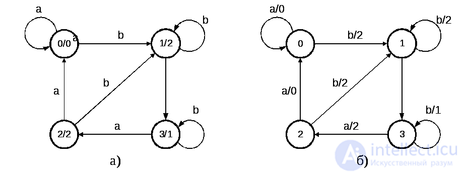Fig. 5.8

The reverse is also true: for any Mile automaton, there is an equivalent Moore automaton. The validity of this statement is easily proved constructively. Consider the Miles machine, shown in Fig. 5.9a. Each state of the Mile automaton is split into several equivalent states, with each of which is associated with one output symbol. For our example, these are the states p0, p1, q0, ql, r0, rl. The construction of transitions of the equivalent Moore automaton is clear from figure 5.9b.

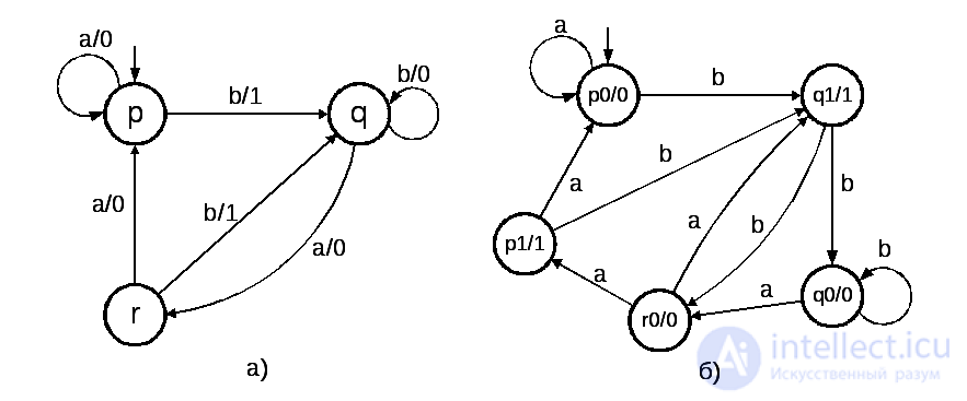Fig. 5.9

Note, however, that this equivalence of the Mily and Moore automata does not reflect their significant difference: the output signals in the Mile automaton are associated with (instantaneous) transition events of the automaton, while the output signals in Moore’s automaton are determined upon entering its new state. In examples of real systems whose operation is described by a model of a finite automaton, the difference between two types of output signals is usually clearly visible - impulse signals that occur only at the moments of system transitions from one state to another, and potential output signals that occur at the moment of entering the state and remain unchanged all the time while the machine is in the current state. In real control systems, both types of signals are often needed. In many applications of finite automata for the specification of discrete systems with memory, functions are used at state transitions, as well as input functions and output functions, which are activated respectively at the moment of entering a new state and leaving the current state