Lecture
There is a concept of chains in graph theory. A bunch of vertices and edges forms a chain in the graph. A chain is called complete if it connects all the vertices of the graph without the formation of loops and contours. The chain has a head and tail . The head of the chain is attached to a vertex, which is called a snap . Chains form paths in a graph.
The path in an undirected graph G is a sequence of edges and vertices L ( v 0, x 1 , v 1 , x 2 , v 2 , x 3 , v 3 , x n , v n ), where v - vertices, x - edges. In this case, the vertex v 0 is called the beginning of the path, and the vertex v n is called the end. Each other vertex is incident to the previous edge and the next, since the end of each edge coincides with the beginning of the next.
The path consisting of one vertex is called zero. A path is called simple if no arc or edge occurs twice in it. A path is called elementary if no vertex is found twice in it.
Cycle - this is a closed path in neorgraph. A cycle in a non-graphgraph is called an Eulerian bypass or an Eulerian cycle if it contains all the edges of the graph exactly once. If there is an Euler cycle in the graph, then such a graph is called Euler. The necessary and sufficient conditions for the existence of the Euler cycle were determined by the great Leonard Euler and in modern terminology are formulated in the following theorem.
Theorem 4.1. An undirected graph is Euler if and only if it is connected and all the degrees of its vertices are even.
Need. The fact that in a disconnected graph there cannot be a cycle passing through all edges is obvious. Suppose now that the graph is connected and there exists an Euler cycle with a beginning at the vertex v 1 . Let's go through this cycle, marking the edges that have been traversed. Through each vertex the cycle can go several times, each time adding two marked edges. During each pass through the vertex v 1, an odd number of edges will be marked (because one edge was marked at the first exit from v 1 ), and when passing through the other vertices, an even number of edges was marked. Therefore, the cycle can end in v 1 only if the degree of v 1 is even (the cycle enters by the last unlabeled edge, and one is added to an odd number of marked edges). In all other vertices, all edges will be marked, that is, the number of marked edges at each vertex will be equal to its degree, which will thus be even.
Adequacy. We show how to construct an Euler cycle in a connected graph whose even degrees of vertices are even. Choose a vertex v 1 and build a path from it in an arbitrary order, marking the edges already passed and including only edges that are not yet marked. At the entrance to the vertex, which is different from them, an odd inline edge is marked, at the exit - even; because of the parity of its degree, it is always possible to exit from it along an unmarked edge. Therefore, our path can only end in v 1 (see the proof of necessity), thus forming a cycle P 1 . If all the edges of the graph are marked, then the desired Euler cycle is constructed. If this is not the case, then for any vertex having incident unmarked edges, the number is even. We will find the first such vertex on the path P 1 (we denote it by v 2 ) and we will build a path from it along unlabeled edges. For the reasons given above (the parity of all degrees and the parity of the number of unlabeled edges), this path can end only in v 2 , forming a cycle P 2 . This cycle is inserted into P 1 at the point v 2 . Get a new cycle of P 12 . If there are unmarked edges left after that, then we build another cycle P 3 and insert it into P 12 . We continue this process of building the cycles P i and inserting them into the already constructed cycle P (12 ... i - 1) until there are no unmarked edges. Ultimately obtained cycle P (12 ... k ) and will be Eulerian.
Theorem 4.2 . An undirected graph is Eulerian if and only if it is connected and is the union of several cycles that do not intersect along edges.
1. Let the graph be Eulerian. Then the Eulerian bypass in it can be constructed by the method described in the previous theorem. This tour is a combination of cycles P 1 , P 2 , ... R k , which do not intersect along edges, since each next cycle contains only unlabeled edges, i.e. edges that are not included in previous cycles.
2. Let the graph be connected and is the union of several cycles that do not intersect along edges. Then any edge of the graph belongs to a cycle. If only one cycle passes through a vertex, then its degree is equal to two. If several cycles pass through a vertex, then, since they do not intersect along edges, each cycle adds exactly two edges to the power of a vertex. Therefore, all vertices of the graph have even degrees and, therefore, the graph is Eulerian.
Hamiltonian problem : In 1859, Sir William Hamilton, the famous Irish mathematician, proposed a children's puzzle in which it was proposed to make a trip to 20 cities, having been in each one more than once. Each city was connected with three neighboring ones, so that the road network formed 30 edges of the dodecahedron (Fig. 4.12). For example, if you start a journey from city a , then you need to finish it in cities e , b or h , otherwise you will not be able to return to city a again.
H 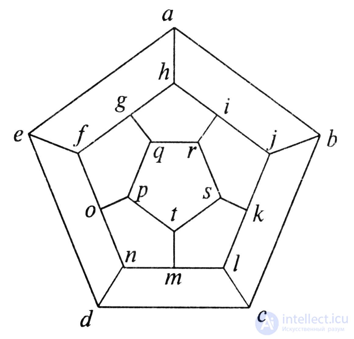 Direct calculation proves that the number of all such routes is 60. For example: - ( abclmtskjirqpondefgh ). From now on, with the light hand of Sir William, any simple path that connects all the vertices of the graph is called Hamiltonian. If there is a simple graph with n vertices, and the degree of each vertex is at least n / 2 , then such a graph will necessarily be Hamiltonian. However, one can easily construct a Hamiltonian graph, whose vertex degree is less than n / 2 .
Fig. 4.12
Paths and connectivity in directed graphs. The path in the oriented graph G O is a sequence of vertices v 0 , v 1 , ... v n , such that v i → v i + 1 for any i , if i + 1 exists.
A number of concepts for undirected graphs — beginning, end, path length, cycle, chain, simple chain — are transferred without change to digraphs. Other concepts, and above all connectivity and accessibility, are significantly modified. It is said that the vertex v j reachable from the vertex v i if there is a path with the beginning in v i and the end in v j . By definition, we assume that any vertex is reachable from itself.
Circuit - this is an oriented cycle in digraph. The concept of simplicity and elementarity applies to both cycles and contours. A contour that contains all the edges or arcs of a graph is called Eulerian. Naturally, the contour that passes all the vertices of the graph without repeating is called Hamiltonian. A connected digraph contains an Euler contour if and only if for each vertex the number of incoming arcs is equal to the number of outgoing ones.
The relation of reachability between vertices in digraphs is asymmetrical: if v j is reachable from v i , then v i is not necessarily reachable from v j .
A half-path in a directed graph is such a sequence of edges, when any two adjacent edges are different and have a common vertex incident to them.
Thus, in graphs there are various types of connectivity, which are described by the following definitions.
1. An orgraph is called strongly connected if any two vertices are reachable from each other (that is, if there are paths between them in both directions).
2. An orgraph is called one-sidedly connected if for any pair of vertices there is a path between them at least in one direction.
3. An orgraph is called weakly connected if there is a half-path between any pair of vertices.
4. An orgraph is called disconnected if there is no half-path between some pair of vertices (i.e., if it is not weakly connected).
The length of the path is the number of edges from the top of v i to the top of v j . The length may be different for the path between the two vertices.
If we consider the path with the minimum number of edges from the vertex v i to the vertex v j , then this path is called the distance r ( v i ; v j ). If there is no path between the vertices, then r = ∞.
The diameter d ( g ) of the graph G is called the maximum distance between its vertices:
d (G) = max d (v i ; v j ).
For any vertex, you can determine the average deviation from the center of the graph by the formula
D ( v i ) = 1 / m ∑ r ( v i ; v ),
where m - the number of arcs in the graph G , and v - runs through all the vertices of the graph.
The vertex for which D ( v i ) is minimal is called the center of the graph. There may be several vertices that are the center.
Maximum removal r ( v i ) from the center of the graph is called the radius of the graph G and is denoted by r ( G ).
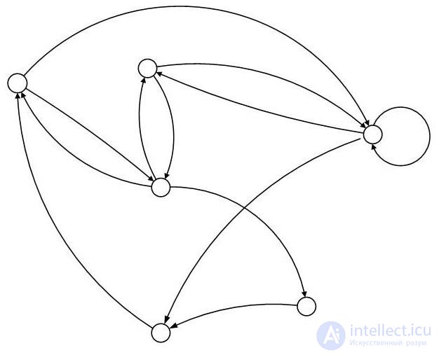
Consider the digraph G 1 with the number of vertices n = 6 and the number of arcs m = 12 , shown in Fig. 4.13.
Construct the matrix R = || r ij ||, which reflects all the distances between the vertices of the graph G 1 . Based on it, you can calculate all possible deviations of the vertices from the center of the graph:
D 1 = 8/12; D 2 = 8/12; D 3 = 9/12; D 4 = 13/12; D 5 = 11/12; D 6 = 7/12.
Thus, the vertex v 6 is the center of the graph G 1 .

 2 1 2 3 4 5 6
1 0 2 1 2 2 1 1
3 2 0 1 2 2 1 2
2 1 0 3 1 2 3
R ( G 1 ) = 2 4 3 0 1 3 4
6 1 3 2 3 0 2 5
1 1 2 1 2 0 6
four
five
Fig. 4.13
To recalculate all possible paths of length r , consider the various degrees of the adjacency matrix of the graph G 1 .


 1 2 3 4 5 6 1 2 3 4 5 6
0 0 1 0 0 1 1 1 2 1 1 1 1 1
0 0 1 0 0 1 2 1 2 1 1 1 0 2
A ( G 1 ) = 0 1 1 0 1 0 3 A2 ( G 1 ) = 1 1 2 0 1 1 3
0 0 0 0 1 0 4 1 0 0 0 0 0 4
1 0 0 0 0 0 5 0 0 1 0 0 1 5
1 1 0 1 0 0 6 0 0 2 0 1 2 6


 1 2 3 4 5 6 1 2 3 4 5 6
1 1 4 0 2 3 1 6 8 18 2 9 12 1
1 1 4 0 2 3 2 6 8 18 2 9 12 2
A3 ( G 1 ) = 2 3 4 1 2 2 3 ... A5 ( G 1 ) = 10 14 19 5 11 10 3
0 0 1 0 0 1 4 1 1 4 0 2 3 4
1 2 1 1 1 0 5 5 7 6 3 4 2 5
3 4 2 2 2 0 6 11 16 13 7 9 4 6
The adjacency matrix A ( G 1 ) gives the number of paths whose length is equal to one arc. The square of the matrix A2 ( G 1 ) gives the number of paths whose length is equal to two. The cube of the matrix A3 ( G 1 ) is the number of paths in three arcs, etc.
There is a notion of the marked adjacency matrix A n ( G 1 ), in which instead of units corresponding vertices are put down, i.e. the marked matrix, in addition to the number of paths, also indicates the vertices through which these paths lie. Then on the diagonal of the marked matrix all possible contours will be indicated, the length of which is determined by the degree of the matrix. The following matrices of the first and second degree are shown below.


 1 2 3 4 5 6 1 2 3 4 5 6
0 0 13 0 0 16 1 161 132 1 1 1 0 1
162
0 0 23 0 0 26 2 261 232 1 1 1 0 2
262
A ( G 1 ) = 0 32 33 0 35 0 3 A2 ( G 1 ) = 351 1 323 0 1 1 3
333
0 0 0 0 45 0 4 451 0 0 0 0 0 4
51 0 0 0 0 0 5 0 0 1 0 0 1 5
61 62 0 64 0 0 6 0 0 613 0 1 616 6
623,626
Non-repeating vertices for individual paths will point to elementary paths. Since graph G 1 has six vertices, then the elementary paths, the length of which would be equal to six arcs, cannot be at all. Thus, the maximum degree of the matrix to determine all Hamiltonian paths must be equal to n - 1 , i.e. five. If in such a matrix we leave only those paths and contours that are Hamiltonian, then we get

 1 2 3 4 5 6
162351 0 0 0 132645 0 1
0 235162 264513 235164 0 0 2
A5 ( G 1 ) = 326451 0 351623 0 0 0 3
0 451623 0 0 0 451326 4
0 0 0 513264 516235 0 5
0 645132 0 0 0 623516 6 .
In our graph G 1 , as the matrix A5 ( G 1 ) shows, there are only three different Hamiltonian paths: 326451, 451623 and 235164. On the diagonal, the same simple contour 162351 is left, which, however, is not Hamiltonian.

Comments
To leave a comment
Finite state machine theory
Terms: Finite state machine theory