Lecture
An automaton can be defined in various ways, for example, by verbally describing its functioning or by listing the elements of the sets X, Y, Q with an indication of the relationships between them. In analyzing and synthesizing finite automata, standard presentation forms are used: tables, graphs, and matrices.
If the elements of the sets X, Y, Q are known, then the characteristic functions δ and λ can be represented by two tables, the rows of which correspond to the internal states of the automaton, and the columns the inputs. Let the internal states of the automaton, q v +1 , be written in the cells of the first table, at which the automaton at a given clock moment τ v passes from the state q v under the influence of the input x v . This table is called the conversion table (Table 5.1). and thus corresponds to the transition function q v +1 = δ ( q v , x v ). In the cells of the second table, the values of the outputs at this clock moment τ v are entered. Such a table is called a table of outputs (Table 5.2) and corresponds to the characteristic function of the outputs y v = λ ( q v , x v ). Examples of such tables for a certain finite state machine with a given input alphabet X = { x 0 , x 1 , x 2 , x 3 }, output alphabet Y = { y 0 , y 1 } and a set of internal states Q = { q 0 , q 1 , q 2 , q 3 } are given below.
Table 5.1 Table 5.2
|
δ |
x 0 |
x 1 |
x 2 |
x 3 |
|
|
λ |
x 0 |
x 1 |
x 2 |
x 3 |
|
q 0 |
q 3 |
q 2 |
q 1 |
q 3 |
|
|
q 0 |
y 0 |
y 0 |
y 0 |
y 0 |
|
q 1 |
q 3 |
q 2 |
q 1 |
q 3 |
|
|
q 1 |
y 1 |
y 0 |
y 0 |
y 1 |
|
q 2 |
q 3 |
q 2 |
q 2 |
q 3 |
|
|
q 2 |
y 1 |
y 0 |
y 1 |
y 1 |
|
q 3 |
q 3 |
q 0 |
q 0 |
q 1 |
|
|
q 3 |
y 0 |
y 0 |
y 1 |
y 1 |
Both tables can be combined into one common transition table , if you place both the internal state and the output value separated by a slash in each cell (we agree in the numerator to record the subsequent internal state of the machine and its current output value in the denominator). Such a table for our machine is presented in table. 5.3.
Table 5.3
|
δ |
x 0 |
x 1 |
x 2 |
x 3 |
|
q 0 |
q 3 / y 0 |
q 2 / y 0 |
q 1 / y 0 |
q 3 / y 0 |
|
q 1 |
q 3 / y 1 |
q 2 / y 0 |
q 1 / y 0 |
q 3 / y 1 |
|
q 2 |
q 3 / y 1 |
q 2 / y 0 |
q 2 / y 1 |
q 3 / y 1 |
|
q 3 |
q 3 / y 0 |
q 0 / y 0 |
q 0 / y 1 |
q 1 / y 1 |
To simplify the filling of the tables, you can write in the cells only the index numbers of the inputs, outputs and states of the machine. Then, for example, the general transition table will look like (Table 5.4):
Table 5.4
|
δ |
0 |
one |
2 |
3 |
|
0 |
3/0 |
2/0 |
1/0 |
3/0 |
|
one |
3/1 |
2/0 |
1/0 |
3/1 |
|
2 |
3/1 |
2/0 |
2/1 |
3/1 |
|
3 |
3/0 |
0/0 |
0/1 |
1/1 |
When analyzing automata, it is convenient to use the language of graphs, which by its clarity makes it easy to transfer many concepts and methods of this theory to automata. In this regard, the most common and illustrative way to represent an automaton is a oriented multigraph, which is also called a transition graph or transition diagram. The vertices of the graph correspond to the states of the automaton and are uniquely labeled with symbols from the set Q (each symbol from Q is used exactly once, as the label of some vertex). Each transition from one state of the automaton to another corresponds to an oriented edge of the graph (arc), generally marked with a symbol from the alphabet X (input) and the symbol of the output alphabet Y (for readability, the elements of the input and output alphabets are separated by a slash). However, it should be noted that not every symbol must be used as a mark and not all arcs must be marked with both symbols.
Multiple edges in the graph are not necessary, they can be replaced by one edge, marked with a disjunction of the corresponding conditions of transitions from one state machine to another. If the transition condition requires more than one input action, then the corresponding arc is marked with a conjunction of all the required inputs.
H  and fig. 5.2 shows a graph constructed in accordance with the transition table above. So if from state 0 the automaton goes to states 1, 2 and 3, then arcs go from vertex 0 of the graph to vertices 1, 2 and 3. At the same time, the transition to state 1 occurs under the influence of input 2 and it corresponds to output 0, therefore the corresponding arc marked as 2/0. The transition to state 2 takes place under the influence of input 1 and it corresponds to output 0, so the arc from vertex 0 to 2 is marked as 1/0. Transitions to state 3 are performed under the influence of inputs 0 and 3, and both of them correspond to output 0, therefore the arc from vertex 0 to 3 is marked as disjunction 0/0 3/0. Other arcs of the graph are defined similarly. Loops correspond to transitions in which the state of the automaton does not change. Thus, the considered automaton passes from state 2 to 2 under the influence of inputs 1 and 2 with outputs 0 and 1. Therefore, the loop at vertex 2 is marked as a disjunction 1/0 2/1. Fig. 5.2
Not every graph can be automaton . For any transition graph at each vertex q i the following conditions must be met, which are called the conditions for the correctness or automatism of the graph:
1. There are no two or more edges with the same characters of the input alphabet x j , emerging from the same vertex q i (consistency or uniqueness condition);
2. For any input letter x j there is an edge that goes from the vertex q i , which is marked with the symbol x j (completeness condition).
Naturally, finite automata are given by finite graphs, and infinite ones - by infinite ones. Example: Consider (Fig. 5.3) an infinite binary tree that converts an input sequence of zeros and ones into an output one. A tree has two types of vertices - 0 and 1, and each edge is labeled with the symbols of entry and exit. Arrows indicate a possible continuation of the branches. The bold line indicates the input sequence x = 1010, which is converted to the output y = 1100.
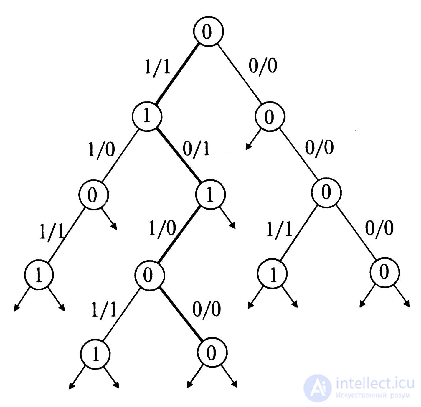

Fig. 5.4
Fig. 5.3
Such an infinite binary tree defines an automaton A, which, depending on the input symbol, can have one of two states 0 or 1. Let the initial state q 0 = 0. If the input of the automaton is x = 0, then the next state of the automaton will be equivalent to the previous one, t . q 1 = 0, and the output will be y = 0. If, on the input, x = 1, the automaton goes to the state q 2 = 1, and the output will be y = 1. Next, being, for example, in the state q 2 , the automaton behaves as follows: if x = 0, then y = 1; if x = 1, then y = 0. In other words, if there is a zero at the input ( x = 0), the state of the outputs does not change, and for x = 1, the state of the outputs changes to the opposite.
The same automaton can be defined using a strongly connected digraph (Fig. 5.4) - a graph, according to which the automaton can go from any state to any other state, bypassing the intermediate ones. The edges of such a graph show transitions from one state of the automaton to another, with the corresponding formation of outputs, and loops - preservation of the previous state and output.
The automaton can be set using a common transition table, vertically arranging the internal states of the automaton, and horizontally the characters of the inputs (Table 5.5).
Finally, an automaton can be specified in analytical form by two functions: the transition function q v +1 = δ ( q v , x v ) and the output function y v = λ ( q v , x v ). For our case, the specific form of these functions will be very simple - the addition of arguments to M2 (the inequality function):
q v +1 = q v x v ; y v = q v x v .
The analyzed automaton has a remarkable property: it reacts to the parity of the units applied to its input. Suppose that the initial state is q 0 = 0, and the input x is an infinite sequence of 0 and 1 (Table 5.6). Then an odd number of units at the input of the automaton A will be marked by units at the output y 0 . If we choose q 1 = 1 as the initial state, then an odd number of ones at the input x will be marked with zeros at the output y 1 .
Table 5.5 Table 5.6
|
q x |
0 |
one |
|
x |
0 0 1 1 0 1 0 0 0 1 0 1 1 ... |
|
0 |
0/0 |
1/1 |
|
y 0 |
0 0 1 0 0 1 1 1 1 0 0 1 0 ... |
|
one |
1/1 |
0/0 |
|
y 1 |
1 1 0 1 1 0 0 0 0 1 1 0 1 ... |
Consider another example of an automaton. Let the transition function take the value of the input symbol ( q v +1 = x v ), and the output function is the state value ( y v = q v ). The general table of transitions of such an automaton is presented in table 5.7, and the formation of the output sequence at different initial states of the automaton depending on the input sequence is shown in table 5.8.
Table 5.7 table 5.8
|
q x |
0 |
one |
|
x |
0 0 1 1 0 1 0 0 0 1 0 1 1 ... |
|
0 |
0/0 |
1/0 |
|
y 0 |
0 0 0 1 1 0 1 0 0 0 1 0 1 ... |
|
one |
0/1 |
1/1 |
|
y 1 |
1 0 0 1 1 0 1 0 0 0 1 0 1 ... |
From tab. 5.8 shows that the automaton at the output, regardless of its initial state, simply shifts all input characters one position to the right. Such a machine is called a delay machine for one clock cycle. Its graph is presented in fig. 5.5. As can be seen in the image of the delay autograph digraph, it has an elementary symmetry group with respect to the state permutation, as well as the input and output symbols 0 and 1.
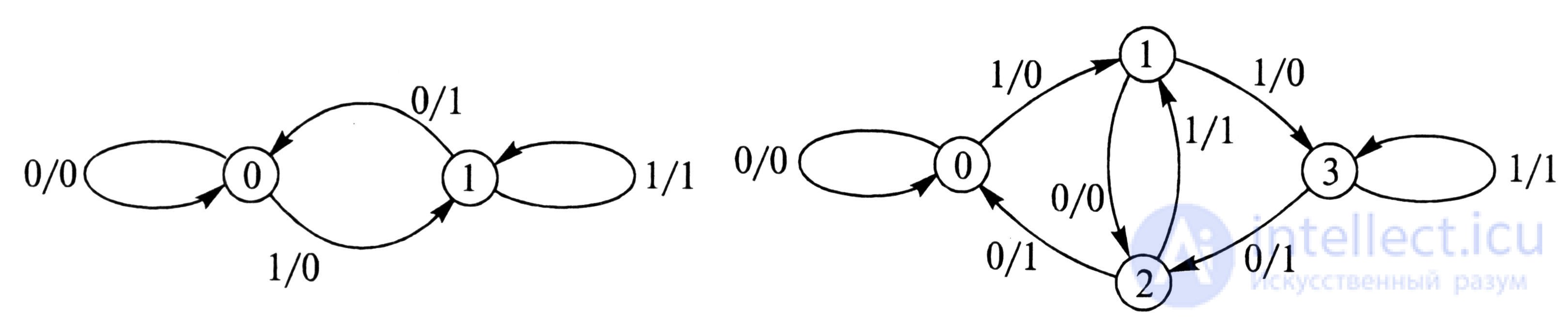
Fig. 5.5 Figure 5.6
You can build an automatic delay for two cycles. Its digraph will also have symmetry properties, although the number of its states will increase to 4, and the number of arcs will increase to 8 (Figure 5.6).

Comments
To leave a comment
Finite state machine theory
Terms: Finite state machine theory