Lecture
The apparatus for describing complex systems of series-parallel processes are formal systems such as Petri nets , which simulate the dynamic properties of systems. The Petri net is a quadruple C = { P, T, I , O }, where P is a finite set of positions , T is a finite set of transitions , I : P → T ∞ - input function that displays the transitions in sets of transitions, O : T → P ∞ - output function that displays the transitions in sets of positions. Graphically, the Petri net is depicted as a multigraph with two types of vertices: the circles correspond to the positions, the bars correspond to the transitions. Functions I and O are represented by arcs (Fig. 5.18).
P 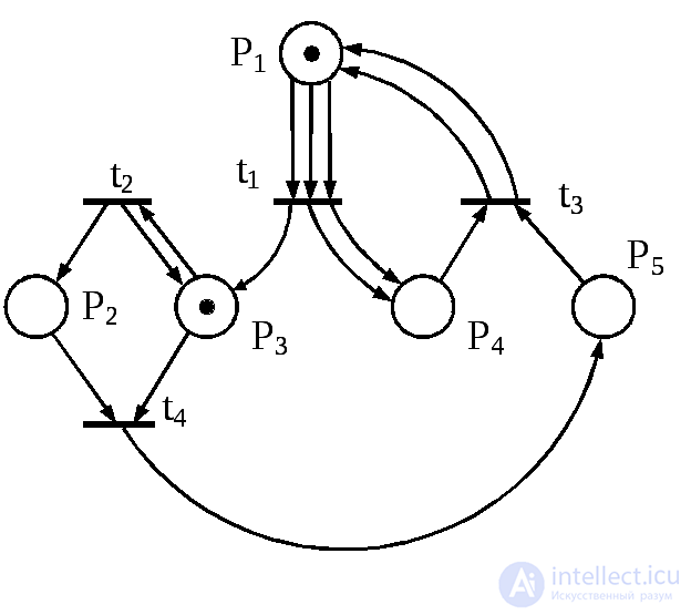 Positions, the arcs from which lead to the transition t j , are called input for t j , similarly to the position, into which the arcs from the transition t j lead, are called output for t j . The set of input positions denote I ( t j ), and the output - O ( t j ). In the Petri network shown in fig. 5.18,
I ( t 1 ) = { p 1 , p 1 , p 1 },
O ( t 1 ) = { p 3 , p 4 , p 4 }.
F
Fig. 5.18
The functions I and O are conveniently generalized to the mapping from positions to sets of transitions ( P → T ∞), which allows us to designate sets of input and output transitions of position p i , defined similarly to sets of input and output transition positions, respectively I ( p i ) and O ( p i ). In the Petri network shown in fig. 5.18, I ( p 3 ) = { t 1 , t 2 }, O ( p 3 ) = { t 2 , t 4 }.
The concepts introduced refer to the static structure of the Petri net. The dynamic properties of the Petri net are determined using the notion of labeling. The marking μ of the Petri net C = ( P, T, I, O ) is a function that maps the set of positions P to the set of non-negative integers N. Marking is depicted with the help of placed inside the positions of chips (points). Thus, the marking of the Petri net shown in Fig. 5.18, is defined as μ ( p 1 ) = μ ( p 3 ) = 1, μ ( p 2 ) = μ ( p 4 ) = μ ( p 5 ) = 0
It is convenient to represent the label as an n- vector μ = (μ 1 , μ 2 , ..., μ n ) (where n = | P | ), each element of which  there is
  and also as a set μ , which includes the network positions p i P and # ( p i , μ ) = μ ( p i ). The Petri Net C with the marking μ defined in it is called a labeled Petri Net.
Network labeling may change as a result of launching transitions . The transition t j of the marked Petri Net C marked μ is allowed if I ( t j ) μ , i.e. there are no fewer chips in each input position t j than arcs from t j come from this position. Any allowed transition may start. As a result of launching the transition t j, the marking of the network μ changes to a new one: μ '= μ - I ( t j ) + O ( t j ), i.e., as many chips as arcs are removed from each input position p i of the transition t i from p i to t j , and in each output position p k there are as many chips as arcs lead from t j to p k . The sequence of launches of transitions is called the execution of the Petri net .
Consider the implementation of the Petri net shown in Fig. 5.18. In the initial labeling only the transition t 2 is allowed. When it is launched, the chip will be removed from p 3 , and then a chip will be added to the p 2 and p 3 positions, i.e., as a result of the launch, a new chip will also appear in p 2 . Now transitions t 2 , t 4 become allowed. Since any transition can start, suppose that the transition t 4 starts. After it is launched from the p 2 and p 3 positions, the chips will be deleted, and one chip will appear in the p 5 position. In the resulting marking μ '' no transition is allowed. This completes the implementation of the Petri net.
Consider the marking μ of the Petri net C = ( P, T, I, O ). Marking μ ' is called directly accessible from μ , if there is such a transition t j  T , allowed in μ , that when it starts up, it is labeled μ ' ; in this case, the pair ( μ , μ ' ) belongs to the ratio of immediate reachability defined on P ∞. This ratio is called reachability ratio . Markings μ ' such that ( μ , μ' ) belong to the reachability relation are called reachable from μ . The set of attainable markings from the Petri net of C is called the reachable set and is denoted by R ( C , μ ).
Interpretation of Petri nets is based on the concepts of condition and event . For the occurrence of an event it is necessary to fulfill certain conditions, called preconditions . The occurrence of an event can lead to a violation of preconditions and to the fulfillment of some other conditions, called post-conditions . In the Petri net, conditions are modeled by positions, events - by transitions. The preconditions of an event are represented by the input positions of the corresponding transition, the postconditions by the output positions. The occurrence of an event is modeled by the launch of the transition. The fulfillment of the conditions is represented by the presence of chips in the respective positions, the non-fulfillment - by their absence.
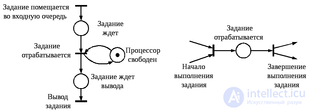
Fig. 5.19
Fig. 5.20
Consider, for example, a simple computing system that sequentially processes jobs that arrive in the input queue. When the processor is free and there is a job in the input queue, it is processed by the processor, then output. This system can be simulated with the Petri net shown in fig. 5.19.
Let us establish what features of the systems Petri nets take into account. This is primarily asynchronous . The concept of time is missing in the Petri net. The time of occurrence of events is not indicated in any way, but, nevertheless, the structure of the Petri net establishes a partial order of occurrence of events. Further, since the occurrence of events is represented by the launch of transitions, it is assumed that events occur instantaneously . If, however, the simulated event has a nonzero duration, such as, for example, the “task is processed” event (Fig. 5.19), and this is significant, then it is represented as two instant events like “event start”, “end of event” and condition “ an event occurs ”(fig. 5.20). In addition, it is believed that events occur at one time (instantaneous events can not occur simultaneously). Indeed, if we assume the simultaneous occurrence of some events i and j , which correspond to transitions t i and t j in the Petri net, then we can introduce an additional transition t ij with I ( t ij ) = I ( t i ) + I ( t j ), O ( t ij ) = O ( t i ) + O ( t j ), interpreted as the simultaneous occurrence of events i and j . In this case, the transitions can be run sequentially.
Petri nets are mainly used as a formal apparatus in modeling systems that are characterized by parallelism. There are two fundamentally different approaches to using Petri nets. In the first, the system is modeled by the Petri net, which is converted according to certain rules to some “optimal” form. In the second, more generally accepted approach, a system project is first created using conventional means and a model is constructed on it in the form of a Petri net. Then, the properties of the resulting network are investigated and conclusions are drawn about the properties and characteristics of the project. This process ends when the Petri net has the necessary properties.
One of the most important tasks of analyzing Petri nets is the problem of reachability : is the marking μ ' from the initial marking μ of this Petri net achievable? The importance of this task is due to the fact that the marking serves as an interpretation of the state of the system. The solution to the reachability problem will allow us to determine whether a particular state is reachable, whether it is “good” or “bad” for the system.
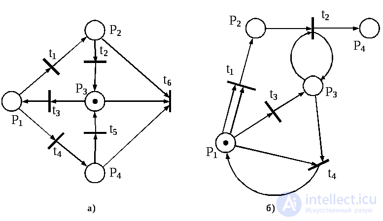
Fig. 5.21
To solve the problems of analysis there are two main approaches. The first is based on building a reachability tree. The reachability tree is an oriented root tree, the vertices of which correspond to possible markings, and to arcs - transitions. The root vertex corresponds to the initial marking. Arcs corresponding to the allowed transitions emanate from each vertex. The tree is built sequentially, starting from the root vertex; at each step is built the next tier of the tree. For example, the reachability tree for the Petri net shown in Fig. 5.21а, after three steps, has the form given in fig. 5.22a (markings are represented by vectors). Obviously, if you do not use certain conventions when building a tree, then active (even limited) Petri nets will have an infinite reachability tree.
(  0,0,1,0) (1,0,0,0)
t3 t1
(1,0,0,0) (1, ω, 0,0)
t1 t4 t1 t3
(0,1,0,0) (0,0,0,1) (1, ω, 0,0) (0, ω, 1.0)
t2 t5 t2
(0,0,1,0) (0, ω, 1, ω)
t2
a) b) (0, ω, 1, ω)
Fig. 5.22
We call vertices (and the corresponding markings) constructed at the next step of the algorithm boundary . If there are no allowed transitions in any boundary marking, then we will call such marking terminal . If any boundary vertex has a label that already exists in the tree, then we call it duplicative . For terminal and duplicate vertices we will not build arcs emanating from them. This ensures the finiteness of the reachability tree for a restricted Petri net (for example, Fig. 5.21a, 5.22a). For unlimited networks, you need to somehow mark an unlimited number of chips in a position. Let ω denote such a number, with ω + a = ω , ω - a = ω , and < ω , ω ≤ ω , where a is an arbitrary positive integer. We will use the following rule when building a reachability tree. Let the boundary vertex μ not be terminal or duplicate. For each allowed transition t j in the marking μ we construct an arc starting from μ . Arc will be marked by the transition t j . The marking μ 'of a new vertex is defined as follows. If a  ( p i ) = ω , then μ ' ( p i ) = ω . If, on the path from the root vertex to μ, there exists a vertex μ ″, such that as a result of the transition into j j j, the number of chips in each position is not less than in μ ″ , and in the position p i is strictly greater, then μ ′ ( p i ) = ω . Otherwise, μ ' ( p i ) is the number of chips in the position p i , which is obtained after launching t j from μ (Fig. 5.22b).
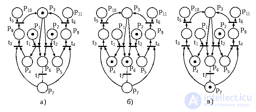
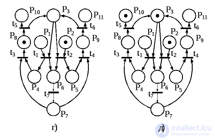
Fig. 5.23
Direct interpretation of the Petri net is possible in two versions: direct and inverse. The inverse variant is that the conditions are associated with the transitions of the network, and the events - with the positions.
The direct option is that the conditions are associated with the positions of the network, and the events - with transitions. Turn to rice. 5.23, which presents a model for servicing the queue of requests from two processes that claim to use some shared resource. A chip in position P1 means that an application has been received from the first process, and a chip in position P2 indicates the arrival of the application from the second process. The presence of chips in position P3 indicates that the resource is free. The initial marking is shown in fig. 5.23a. Suppose that the application from the first process arrived a little earlier. In this case, the transition t1 is triggered. This means that the first process is selected from the queue to the resource, after which the marking shown in Fig. 3 is achieved. 5.23b.
The next step is the transition t7, and within the framework of the transition the first process uses the resource allocated to it, and the next marking will be the one shown in fig. 5.23c. In this situation, there are conditions for the operation of the transition t3. This triggering means that the first process processes the results associated with the use of the resource, and the new marking takes the form shown in Fig. 5.23g.
Now there are conditions for the release of the resource by the first process: the transition t5 is triggered. The marking achieved at the same time (Fig. 5.23d) means that the second process can use the resource. This completes the cycle of the first process. We describe it in terms of events and conditions.
Event t 1 . Action: Select the first process from the queue to the resource.
Precondition: Р1 - there is an application from the first process; P3 - the resource is free.
Postcondition: P4, P6 - the application of the first process is completed.
Event t 7 . Action: use the first process of the resource.
Precondition: P6 - the application of the first process is completed.
Postcondition: P7 - results from the use of the first process of the resource obtained.
Event t 3 . Action: processing the results associated with the use of the resource.
Precondition: Р4 - the application of the first process is completed; P7 - results from the use of the first process of the resource obtained.
Postcondition: P8 - processing of the results associated with the use of the resource is completed.
Event t 5 . Action: release by the first process of the resource.
Precondition: Р8 - processing of the results associated with the use of the resource is completed.
Postcondition: Р10 - the first process has completed the cycle of its work; P3 - the resource is free.
In the inverse version of the Petri net, the positions correspond to the operations (i.e. events) of the process being implemented, and the transitions correspond to the conditions (i.e. states) of the change of operations. The transition corresponds to the operator formula of the form
Z ( t ) = F ( x l ( t ), ..., x n ( t )),
where Z ( t ) is the output logical variable; F - operator; x i ( t ), i = 1, n - input logical variables.
The truth of the output logical variable is a necessary condition for the transition to be triggered.
Control tasks
1. Build a state machine that sells beer and gives change. The machine can accept coins of 5 and 10 pence, and a beer mug costs 15 pence. In addition to the holes for accepting coins and issuing change, the machine has “Fill” and “Reset” buttons.
2. Build a spacecraft throwing out all comments from a C program, taking into account possible string constants, which, of course, cannot be changed. A comment in the C language is any string bounded by complex brackets: / * ... * / or a pair of slashes // and the end of the line. Constant characters may appear inside a string constant. They are entered with double quotes.
3. Build a spacecraft, issuing the remainder of dividing the decimal number entered by 3.
4. Construct the spacecraft, issuing the result of dividing the entered 5-number number by 3. The result is given in the form: (). The number is entered from the upper digits and ends with a “#” end marker. The result is also represented in the five-fold number system.
5. Construct a spacecraft, issuing the remainder of dividing the input ternary number by 4. Construct two variants of the automaton: for the case when the number is entered from the upper digits, and for the case when the number is entered from the lower digits.
6. Build a spacecraft emitting extra spaces in the text.
7. Build a QA that adds an odd bit to the chain of 0 and 1.
8. Construct Moore's submachine gun, which controls the traffic light of the automatic control of transport at a regular intersection. Note that in one direction the movement is allowed for t1 seconds, and in the other direction - t 2 seconds.
Note. The only input event of the machine is the timeout event. Therefore, it is an autonomous machine that generates a cyclic sequence of outputs.
9. (Automatic traffic light). Solve the problem of regulating transport at the T-junction (Fig. 5.24), where the main stream of transport goes from west to east, and a secondary road comes from the south.
H 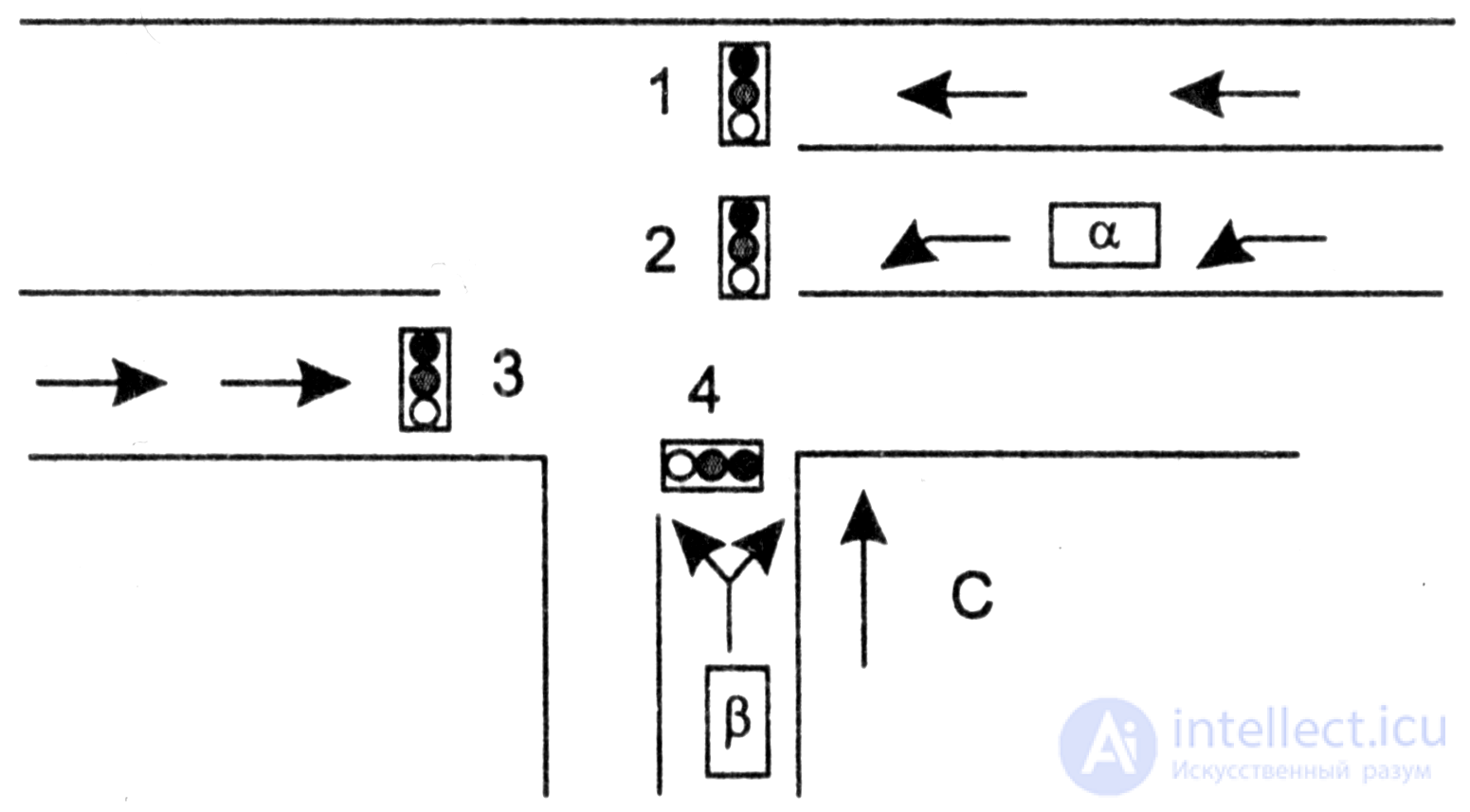 Four traffic lights control the traffic, each can show one of three signals: K , F , 3 . Obviously, they should be managed in a coordinated manner so that an emergency situation is not created (for example, there would be no “Green” signal at all four traffic lights). The control unit generates four signals, for example, <К; 3; Ж; 3> - at the first traffic light red, at the second and fourth - green, and at the third - yellow. Fig. 5.24
Considering that transport in the direction of the secondary road rarely moves, build a Moore finite automaton that controls the intersection for transport requests. Transport requests are automatically transmitted using sensors α and β . On these sensors, a value of 1 is set if a car appears in the appropriate place. The inputs to the control unit are the pairs <0,0>; <0.1>; <1.0>; <1,1> sensor states ( α and β , and exits - four signals of traffic lights.

Comments
To leave a comment
Finite state machine theory
Terms: Finite state machine theory