Lecture
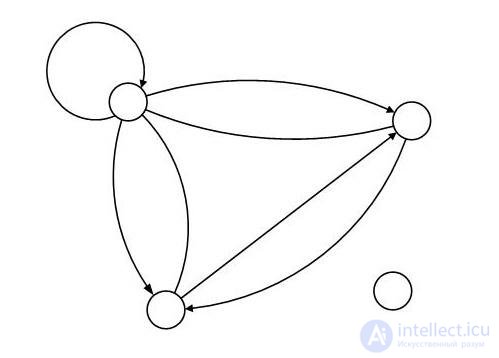
Consider an example of constructing a graph. Let the set of vertices be defined as V = {a, b, c, d}, and the set of edges as X = {1, 2, 3, ..., 7}. Let the incidentor of the graph P be defined by nine values: P (a, 1, a); P (a, 2, b); P (b, 3, a); P (a, 3, b); P (a, 4, c); P (a, 5, c); P (c, 5, a); P (c, 6, b); P (b, 7, c) - which are true, the rest are false. The image of the graph is presented in Fig. 4.8. In this example, the vertices a, b, and c are adjacent, and the vertex d is isolated, i.e. not incident to any edge.
 one
one
2
but
3 b
4 5
6
7
d
c
Fig. 4.8
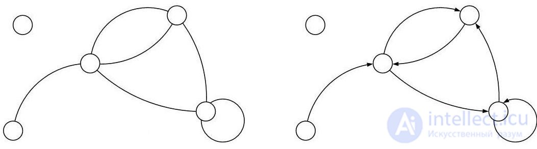
There are other ways to define graphs. Let us consider another example: let an image of an undirected graph G (Fig. 4.9a) and a similar digraph G O (Fig. 4.9b) be given. Let v 1 , v 2 , ... v 5 - vertices, and x 1 , x 2 ... x 6 - edges (arcs). The graphs G and G O can be represented in analytical form either by the adjacency matrix A or the incidence matrix B.
 v 4 x 2 v 3 v 4 x 2 v 3
x 3 x 5 x 3 x 5
x 1 v 2 x 4 x 1 v 2 x 4
v 5 x 6 v 5 x 6
v 1 v 1
a) b)
Fig. 4.9
The incidence matrix of a graph G is the matrix B = || b ij ||, having i = 1, .., n columns and j = 1, ..., m lines, which corresponds to the number of vertices n and the number of edges m. The element of the matrix bij = 1 if the vertex v i is incident to the edge x j , and bij = 0 if not incident. For a directed graph, the element of the matrix is bij = 1 if the arc comes from a vertex, and bij = –1 if the arc comes to a vertex. If there is a loop in the digraph, then bij = 2. For the undirected graph and digraph presented in Fig. 4.9a and b, the incidence matrices are respectively as follows:


 v 1 , v 2 v 3 v 4 , v 5 v 1 , v 2 v 3 v 4 , v 5
1 1 0 0 0 x 1 1 -1 0 0 0 x 1
0 1 1 0 0 x 2 0 1 -1 0 0 x 2
B ( g ) = 0 1 1 0 0 x 3 B ( G O ) = 0 -1 1 0 0 x 3
0 1 0 0 1 x 4 0 1 0 0 -1 x 4
0 0 1 0 1 x 5 0 0 -1 0 1 x 5
0 0 0 0 1 x 6 0 0 0 0 2 x 6
In each row of the incidence matrix, only two elements (or one) are non-zero. The incidence matrix can be used to determine the degrees of all vertices of the graph. At the same time for loops value doubles.
The adjacency matrix of a graph G is called the square matrix A = || a ij ||, columns and rows of which correspond to the vertices of the graph i = 1, ..., n ; j = 1, ..., n . For an undirected graph, the element of the matrix a ij is equal to the number of edges incident to the vertices v i and v j , for a digraph it is equal to the number of edges with the beginning at the vertex v i and the end at the vertex v j . For our example, adjacency matrices will be


 v 1 , v 2 v 3 v 4 , v 5 v 1 , v 2 v 3 v 4 , v 5
0 1 0 0 0 v 1 0 0 0 0 0 v 1
1 0 2 0 1 v 2 1 0 1 0 0 v 2
A (G) = 0 2 0 0 1 v 3 A (G O ) = 0 1 0 0 1 v 3
0 0 0 0 0 v 4 0 0 0 0 0 v 4
0 1 1 0 1 v 5 0 1 0 0 1 v 5
As can be seen, the adjacency matrix for a undirected graph is symmetric, but optional for a digraph. A graph with a symmetric adjacency matrix canonically corresponds to a non-graph with the same adjacency matrix.
So, graphs can be defined in three ways:
1. Directly specifying the sets of vertices V and edges X, as well as the incidence relation.
2. The adjacency matrix or incidence matrix.
3. Graphic image (picture).
How to determine that these two graphs are the same? For the first two ways of setting the answer, the answer is simple: when their descriptions are the same - lists of vertices and edges or matrices. By drawing it is more difficult to determine if the graphs are the same. The same graph can be represented by different patterns (Fig. 4.10), by arranging the vertices in different ways and giving the edges a different geometric shape and length. On the other hand, two seemingly identical patterns can have different graphs if they have different vertex numbers, which is why the adjacency matrices and the lists of edges will be different (Fig. 4.11).
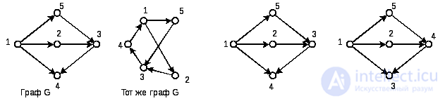
Fig. 4.10 Fig. 4.11
Graphs that differ only in the numbering of the vertices (and which can be made the same by renumbering) are called isomorphic . The isomorphism of graphs with a small number of vertices is sometimes obvious. However, in the general case, the problem of establishing isomorphism of graphs turns out to be a computationally difficult task.

Comments
To leave a comment
Finite state machine theory
Terms: Finite state machine theory