Statistical analysis in PostgreSQL using PL / R

The objective of this publication is to introduce you to the capabilities of the PL / R language. I hope that you find the information presented here useful for you.

PL/R (Programming Language/Relational) is a procedural language extension for the PostgreSQL database system. It allows you to write functions and procedures using the R programming language within the context of a PostgreSQL database. PL/R can be used to perform complex data analysis and statistical computations directly within the database, leveraging the power of R's statistical and analytical capabilities.

Here are some key features and capabilities of PL/R:

1. R Integration: PL/R allows you to write database functions and procedures using the R programming language. This enables you to perform data analysis, modeling, and statistical computations using R's extensive libraries and functions.

2. Data Analysis: With PL/R, you can create stored procedures that perform various types of data analysis directly within the database. This can include tasks such as regression analysis, clustering, data visualization, and more.

3. Statistical Functions: You can define custom statistical functions in R and call them from SQL queries, allowing you to compute statistical measures and summaries on your data.

4. Data Transformation: PL/R can be used to preprocess and transform data stored in the database. This includes cleaning, filtering, and reshaping data before performing analysis.

5. Parallel Processing: PL/R can take advantage of parallel processing capabilities offered by PostgreSQL, allowing you to distribute computations across multiple processors or cores.

6. Scalability: Since PL/R operates within the PostgreSQL database, it benefits from PostgreSQL's scalability features, such as support for large datasets, indexing, and query optimization.

7. Integration with SQL: PL/R functions can be seamlessly integrated with SQL queries. This means you can use SQL to query and manipulate your data and call PL/R functions for more complex analysis tasks.

8. Custom Aggregates: PL/R allows you to create custom aggregate functions that can be used in SQL queries. These aggregates can perform specialized statistical operations on groups of data.

9. Machine Learning: You can leverage R's machine learning libraries to build and apply predictive models within the database.

Keep in mind that while PL/R provides powerful capabilities for data analysis and statistical computations, it might require a good understanding of both SQL and R to effectively utilize its features. It's important to carefully design your functions and procedures to optimize performance and leverage the strengths of both PostgreSQL and R.

Please note that my knowledge is based on information available up to September 2021, and there might have been developments or changes since then. If you're interested in using PL/R, I recommend referring to the official PostgreSQL documentation and resources for the most up-to-date information.

Recent trends in Big Data have encouraged analytics and data convergence, while PL / R has unobtrusively been providing this service for 12 years now! If suddenly you do not know, PL / R is an extension for PostgreSQL that allows you to use R, a language for mathematical calculations, directly from PostgreSQL in order to easily and easily get expanded analytics. Expansion is available and actively improved since 2003. It works with all supported versions of PostgreSQL and with all the latest versions of R. Thousands of people around the world have already appreciated its convenience and efficiency. Let us see what PL / R is, discuss the advantages and disadvantages of such an approach to data analysis and consider several examples for clarity.

To begin with, we will define the basic concepts. R is a programming language for statistical data processing and graphics, as well as a free open-source computing environment. And PostgreSQL is a powerful free object-relational database management system that has been actively developed for more than 25 years and has earned an excellent reputation for its reliability, as well as data correctness and integrity. And finally, PL / R. As mentioned above, this is a procedural R language handler for PostgreSQL, which allows writing SQL functions on R.

So what are the benefits of PL / R? Firstly, PL / R contributes to the development of human knowledge and skills, since mathematics, statistics, databases and the web are different specializations, but all of them will have to be mastered in one way or another to work with PL / R. Secondly, this extension stimulates the improvement of hardware, because you need a server that can withstand the analysis of large data sets. Third, processing efficiency will increase, since you no longer have to transfer large data sets across the entire network, and throughput will increase. Fourth, you can be sure that the analysis will be carried out consistently. Fifth, PL / R makes the system of any complexity understandable and supported. And finally, thanks to the rich functionality and a huge PL / R ecosystem, it expands the possibilities of R.

But, of course, there are downsides. The PostgreSQL user will most likely find that PL / R is slower, especially on simple tasks. And for the R programmer, the debugging process becomes more complicated and the analysis becomes less flexible. In addition, both will have to learn a new language.

Something like this is the standard function in R:

func_name <- function(myarg1 [,myarg2...]) { function body referencing myarg1 [, myarg2 ...] } 

Creating functions in PL / R is somewhat different, but similar to other PLs in PostgreSQL:

 CREATE OR REPLACE FUNCTION func_name(arg-type1 [, arg-type2 ...]) RETURNS return-type AS $$ function body referencing arg1 [, arg2 ...] $$ LANGUAGE 'plr'; CREATE OR REPLACE FUNCTION func_name(myarg1 arg-type1 [, myarg2 arg-type2 ...]) RETURNS return-type AS $$ function body referencing myarg1 [, myarg2 ...] $$ LANGUAGE 'plr'; 

Let's give an example:

 CREATE EXTENSION plr; CREATE OR REPLACE FUNCTION test_dtup(OUT f1 text, OUT f2 int) RETURNS SETOF record AS $$ data.frame(letters[1:3],1:3) $$ LANGUAGE 'plr'; SELECT * FROM test_dtup(); f1 | f2 ----+---- a | 1 b | 2 c | 3 (3 rows) 

It’s hard to list all the things you can do with PL / R, but let's take a closer look at some important features, such as:

• PostgreSQL compatibility;
• custom SQL aggregates;
• window functions;
• translation of the object R to bytea (binary strings).

Due to PostgreSQL compatibility, we can create prototypes using R, and then move to PL / R for production in production. Also undoubted advantage is that all queries are executed in the current database. The driver and connection settings are ignored, so dbDriver, dbConnect, dbDisconnect and dbUnloadDriver do not require extra effort:

 dbDriver(character dvr_name) dbConnect(DBIDriver drv, character user, character password, character host, character dbname, character port, character tty, character options) dbSendQuery(DBIConnection conn, character sql) fetch(DBIResult rs, integer num_rows) dbClearResult (DBIResult rs) dbGetQuery(DBIConnection conn, character sql) dbReadTable(DBIConnection conn, character name) dbDisconnect(DBIConnection conn) dbUnloadDriver(DBIDriver drv) 

Let's give a couple of examples for clarity. Suppose we need to contact PostgreSQL from R to solve the famous traveling salesman problem, which we will look at in detail later:

 tsp_tour_length<-function() { require(TSP) require(fields) require(RPostgreSQL) drv <- dbDriver("PostgreSQL") conn <- dbConnect(drv, user="postgres", dbname="plr", host="localhost") sql.str <- "select id, st_x(location) as x, st_y(location) as y, location from stands" waypts <- dbGetQuery(conn, sql.str) dist.matrix <- rdist.earth(waypts[,2:3], R=3949.0) rtsp <- TSP(dist.matrix) soln <- solve_TSP(rtsp) dbDisconnect(conn) dbUnloadDriver(drv) return(attributes(soln)$tour_length) } 

This is the same function in PL / R:

 CREATE OR REPLACE FUNCTION tsp_tour_length() RETURNS float8 AS $$ require(TSP) require(fields) require(RPostgreSQL) drv <- dbDriver("PostgreSQL") conn <- dbConnect(drv, user="postgres", dbname="plr", host="localhost") sql.str <- "select id, st_x(location) as x, st_y(location) as y, location from stands" waypts <- dbGetQuery(conn, sql.str) dist.matrix <- rdist.earth(waypts[,2:3], R=3949.0) rtsp <- TSP(dist.matrix) soln <- solve_TSP(rtsp) dbDisconnect(conn) dbUnloadDriver(drv) return(attributes(soln)$tour_length) $$ LANGUAGE 'plr' STRICT; 

This is what R finally displays to us:

 tsp_tour_length() [1] 2804.581 

And the same function in PL / R:

 SELECT tsp_tour_length(); tsp_tour_length ------------------ 2804.58129355858 (1 row) 

As you can see, the result is the same.

Now let's talk about aggregates. One of the most useful features of PostgreSQL is the ability to write your own aggregate functions. PostgreSQL aggregates can be extended with SQL commands. At the same time, the state transition function and, sometimes, the final function (final function) are indicated. The initial condition of the transition function can also be specified. And these benefits you can enjoy working with PL / R.

Let us give an example of the function PL / R implementing a new unit. Until recently, it was impossible to do from PostgreSQL, GROUPING SETS functionality appeared only in version 9.5, while PL / R allows it to be done in any version of PG. I will create an aggregate function based on the real data of one production company and call it quartile:

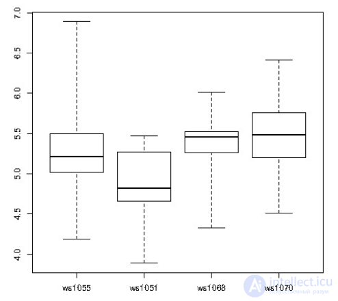
 CREATE OR REPLACE FUNCTION r_quartile(ANYARRAY) RETURNS ANYARRAY AS $$ quantile(arg1, probs = seq(0, 1, 0.25), names = FALSE) $$ LANGUAGE 'plr'; CREATE AGGREGATE quartile (ANYELEMENT) ( sfunc = array_append, stype = ANYARRAY, finalfunc = r_quantile, initcond = '{}' ); SELECT workstation, quartile(id_val) FROM sample_numeric_data WHERE ia_id = 'G121XB8A' GROUP BY workstation; workstation | quantile -------------+--------------------------------- 1055 | {4.19,5.02,5.21,5.5,6.89} 1051 | {3.89,4.66,4.825,5.2675,5.47} 1068 | {4.33,5.2625,5.455,5.5275,6.01} 1070 | {4.51,5.1975,5.485,5.7575,6.41} (4 rows) 

R allows you to display data in the form of nice graphs. In this case, the box diagram was used:

The schedule shows that one of the production stations is less productive than the others, and measures need to be taken to fix this.

Separately it is worthwhile to dwell on window functions (window functions). They are available in PostgreSQL, starting with version 8.4, and are great for statistical analysis. Window functions are similar to aggregate ones, but, unlike them, they do not group rows, but allow calculations to be performed in rowsets associated with the current row, having access not only to the current row of the query result. In other words, your data is divided into sections, and there is a window that slides through these sections and gives the result for each data group:


Few PostgreSQL procedural languages ​​support windowing functions, but they are quite useful in PL / R. Let us give an example: create a table of random data that simulates income and stock prices.

 CREATE TABLE test_data ( fyear integer, firm float8, eps float8 ); INSERT INTO test_data SELECT (bf + 1) % 10 + 2000 AS fyear, floor((b.f+1)/10) + 50 AS firm, f::float8/100 + random()/10 AS eps FROM generate_series(-500,499,1) b(f); CREATE OR REPLACE FUNCTION r_regr_slope(float8, float8) RETURNS float8 AS $BODY$ slope <- NA y <- farg1 x <- farg2 if (fnumrows==9) try (slope <- lm(y ~ x)$coefficients[2]) return(slope) $BODY$ LANGUAGE plr WINDOW; 

And we will write a function to find out whether it is possible to predict revenues this year, based on last year’s figures, using a simple regression method.

 SELECT *, r_regr_slope(eps, lag_eps) OVER w AS slope_R FROM ( SELECT firm AS f, fyear AS fyr, eps, lag(eps) OVER (PARTITION BY firm ORDER BY firm, fyear) AS lag_eps FROM test_data ) AS a WHERE eps IS NOT NULL WINDOW w AS (PARTITION BY firm ORDER BY firm, fyear ROWS 8 PRECEDING); f | fyr | eps | lag_eps | slope_r ---+------+-------------------+-------------------+------------------- 1 | 1991 | -4.99563754182309 | | 1 | 1992 | -4.96425441872329 | -4.99563754182309 | 1 | 1993 | -4.96906093481928 | -4.96425441872329 | 1 | 1994 | -4.92376988714561 | -4.96906093481928 | 1 | 1995 | -4.95884547665715 | -4.92376988714561 | 1 | 1996 | -4.93236254784279 | -4.95884547665715 | 1 | 1997 | -4.90775520844385 | -4.93236254784279 | 1 | 1998 | -4.92082695348188 | -4.90775520844385 | 1 | 1999 | -4.84991340579465 | -4.92082695348188 | 0.691850614092383 1 | 2000 | -4.86000917562284 | -4.84991340579465 | 0.700526929134053 

As you can see, the function considered the dependence of income on indicators of previous years.

The last thing worth talking about in detail is the mechanisms for returning R objects and the methods of their storage.

Let's give an example with stock data. To do this, take the Hi-Low-Close data from Yahoo for any “ticker” (stock ticker). Construct a graph with Bollinger lines and volume. We will need additional R packages that can be obtained from R with the following command:

 install.packages(c('xts','Defaults','quantmod','cairoDevice','RGtk2')) 

Now we will make a query:

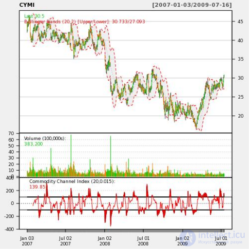
 CREATE OR REPLACE FUNCTION plot_stock_data(sym text) RETURNS bytea AS $$ library(quantmod) library(cairoDevice) library(RGtk2) pixmap <- gdkPixmapNew(w=500, h=500, depth=24) asCairoDevice(pixmap) getSymbols(c(sym)) chartSeries(get(sym), name=sym, theme="white", TA="addVo();addBBands();addCCI()") plot_pixbuf <- gdkPixbufGetFromDrawable(NULL, pixmap, pixmap$getColormap(),0, 0, 0, 0, 500, 500) buffer <- gdkPixbufSaveToBufferv(plot_pixbuf, "jpeg", character(0), character(0))$buffer return(buffer) $$ LANGUAGE plr; 

A typical server will require a screen buffer to create a graph:

 Xvfb :1 -screen 0 1024x768x24 export DISPLAY=:1.0 

Now call the PHP function for the CYMI ticker:

And here is the schedule we get at the output:


Agree, it is surprising that we can write a dozen lines on PL / R and less than a dozen lines in PHP, and eventually get such a detailed visual display and analysis of our data.

To consolidate information, consider more complex examples. I think many are familiar with Benford's law, or the law of the first digit, which describes the probability of the occurrence of a certain first significant digit in the distributions of values ​​taken from real life. But some do not know about its existence and themselves distribute the data as they need, instead of applying the law.

Benford's law can be used to identify potential fraud: it can be used to construct an approximate geometric sequence based on several initial values, and then compare it with real data and find inconsistencies. This method can be applied to sales schedules, census data, cost reports, etc.

Let's look at an example with data from the California Energy Optimization Program. To begin with, we will create and fill in a table with data on investment in the project (data are available at http://open-emv.com/data):

 CREATE TABLE open_emv_cost(value float8, district int); COPY open_emv_cost FROM 'open-emv.cost.csv' WITH delimiter ','; 

Now we write the function of Benford's law:

 CREATE TYPE benford_t AS ( actual_mean float8, n int, expected_mean float8, distorion float8, z float8 ); CREATE OR REPLACE FUNCTION benford(numarr float8[]) RETURNS benford_t AS $$ xcoll <- function(x) { return ((10 * x) / (10 ^ (trunc(log10(x))))) } numarr <- numarr[numarr >= 10] numarr <- xcoll(numarr) actual_mean <- mean(numarr) n <- length(numarr) expected_mean <- (90 / (n * (10 ^ (1/n) - 1))) distorion <- ((actual_mean - expected_mean) / expected_mean) z <- (distorion / sd(numarr)) retval <- data.frame(actual_mean,n,expected_mean,distorion,z) return(retval) $$ LANGUAGE plr; 

And run the comparison:

 SELECT * FROM benford(array(SELECT value FROM open_emv_cost)); -[ RECORD 1 ]-+---------------------- actual_mean | 38.1936561918275 n | 240 expected_mean | 38.8993031865999 distorion | -0.0181403505195804 z | -0.000984036908080443 

It seems that the real data are predictable, so there are no signs of fraud in this case.

Let's return to the traveling salesman problem. This is one of the most well-known problems of combinatorial optimization, which consists in finding the most profitable route that passes at least once through the specified cities, and then returns to the source city. In terms of the task, the criteria for the profitability of the route (the shortest, cheapest, aggregate criterion, and so on) and the corresponding matrices of distances, cost, and the like are indicated. As a rule, it is indicated that the route should pass through each city only once. Let's look at exactly this option.

To begin with, we will create and fill a table with all the cities that need to be visited:

 CREATE TABLE stands ( id serial primary key, strata integer not null, initage integer ); SELECT AddGeometryColumn('','stands','boundary','4326','MULTIPOLYGON',2); CREATE INDEX "stands_boundary_gist" ON "stands" USING gist ("boundary" gist_geometry_ops); SELECT AddGeometryColumn('','stands','location','4326','POINT',2); CREATE INDEX "stands_location_gist" ON "stands" USING gist ("location" gist_geometry_ops); INSERT INTO stands (id,strata,initage,boundary,location) VALUES ( 1,1,1, GeometryFromText( 'MULTIPOLYGON(((59.250000 65.000000,55.000000 65.000000,55.000000 51.750000, 60.735294 53.470588, 62.875000 57.750000, 59.250000 65.000000 )))', 4326 ), GeometryFromText('POINT( 61.000000 59.000000 )', 4326) ), ( 2,2,1, GeometryFromText( 'MULTIPOLYGON(((67.000000 65.000000,59.250000 65.000000,62.875000 57.750000, 67.000000 60.500000, 67.000000 65.000000 )))', 4326 ), GeometryFromText('POINT( 63.000000 60.000000 )', 4326 ) ), ( 3,3,1, GeometryFromText( 'MULTIPOLYGON(((67.045455 52.681818,60.735294 53.470588,55.000000 51.750000, 55.000000 45.000000, 65.125000 45.000000, 67.045455 52.681818 )))', 4326 ), GeometryFromText('POINT( 64.000000 49.000000 )', 4326 ) ) ; 

To get the result, I have to write a couple of auxiliary queries. The first will create a route that I want to get at the output:

 INSERT INTO stands (id,strata,initage,boundary,location) VALUES ( 4,4,1, GeometryFromText( 'MULTIPOLYGON(((71.500000 53.500000,70.357143 53.785714,67.045455 52.681818, 65.125000 45.000000, 71.500000 45.000000, 71.500000 53.500000 )))', 4326 ), GeometryFromText('POINT( 68.000000 48.000000 )', 4326) ), ( 5,5,1, GeometryFromText( 'MULTIPOLYGON(((69.750000 65.000000,67.000000 65.000000,67.000000 60.500000, 70.357143 53.785714, 71.500000 53.500000, 74.928571 54.642857, 69.750000 65.000000 )))', 4326 ), GeometryFromText('POINT( 71.000000 60.000000 )', 4326) ), ( 6,6,1, GeometryFromText( 'MULTIPOLYGON(((80.000000 65.000000,69.750000 65.000000,74.928571 54.642857, 80.000000 55.423077, 80.000000 65.000000 )))', 4326 ), GeometryFromText('POINT( 73.000000 61.000000 )', 4326) ), ( 7,7,1, GeometryFromText( 'MULTIPOLYGON(((80.000000 55.423077,74.928571 54.642857,71.500000 53.500000, 71.500000 45.000000, 80.000000 45.000000, 80.000000 55.423077 )))', 4326 ), GeometryFromText('POINT( 75.000000 48.000000 )', 4326) ), ( 8,8,1, GeometryFromText( 'MULTIPOLYGON(((67.000000 60.500000,62.875000 57.750000,60.735294 53.470588, 67.045455 52.681818, 70.357143 53.785714, 67.000000 60.500000 )))', 4326 ), GeometryFromText('POINT( 65.000000 57.000000 )', 4326) ) ; 

And the second is the data that I enter into the plr_modules, and the type of the resulting data:

 DROP TABLE IF EXISTS events CASCADE; CREATE TABLE events ( seqid int not null primary key, -- visit sequence # plotid int, -- original plot id bearing real, -- bearing to next waypoint distance real, -- distance to next waypoint velocity real, -- velocity of travel, in nm/hr traveltime real, -- travel time to next event loitertime real, -- how long to hang out totaltraveldist real, -- cummulative distance totaltraveltime real -- cummulaative time ); SELECT AddGeometryColumn('','events','location','4326','POINT',2); CREATE INDEX "events_location_gist" ON "events" USING gist ("location" gist_geometry_ops); CREATE TABLE plr_modules ( modseq int4 primary key, modsrc text ); 

Create the main function PL / R:

 CREATE OR REPLACE FUNCTION solve_tsp(makemap bool, mapname text) RETURNS SETOF events AS $$ require(TSP) require(fields) sql.str <- "select id, st_x(location) as x, st_y(location) as y, location from stands;" waypts <- pg.spi.exec(sql.str) dist.matrix <- rdist.earth(waypts[,2:3], R=3949.0) rtsp <- TSP(dist.matrix) soln <- solve_TSP(rtsp) tour <- as.vector(soln) pg.thrownotice( paste("tour.dist=", attributes(soln)$tour_length)) route <- make.route(tour, waypts, dist.matrix) if (makemap) { make.map(tour, waypts, mapname) } return(route) $$ LANGUAGE 'plr' STRICT; 

Now we need to set the function make.route ():

 INSERT INTO plr_modules VALUES ( 0, $$ make.route <-function(tour, waypts, dist.matrix) { velocity <- 500.0 starts <- tour[1:(length(tour))-1] stops <- tour[2:(length(tour))] dist.vect <- diag( as.matrix( dist.matrix )[starts,stops] ) last.leg <- as.matrix( dist.matrix )[tour[length(tour)],tour[1]] dist.vect <- c(dist.vect, last.leg ) delta.x <- diff( waypts[tour,]$x ) delta.y <- diff( waypts[tour,]$y ) bearings <- atan( delta.x/delta.y ) * 180 / pi bearings <- c(bearings,0) for( i in 1:(length(tour)-1) ) { if( delta.x[i] > 0.0 && delta.y[i] > 0.0 ) bearings[i] <- bearings[i] if( delta.x[i] > 0.0 && delta.y[i] < 0.0 ) bearings[i] <- 180.0 + bearings[i] if( delta.x[i] < 0.0 && delta.y[i] > 0.0 ) bearings[i] <- 360.0 + bearings[i] if( delta.x[i] < 0.0 && delta.y[i] < 0.0 ) bearings[i] <- 180 + bearings[i] } route <- data.frame(seq=1:length(tour), ptid=tour, bearing=bearings, dist.vect=dist.vect, velocity=velocity, travel.time=dist.vect/velocity, loiter.time=0.5) route$total.travel.dist <- cumsum(route$dist.vect) route$total.travel.time <- cumsum(route$travel.time+route$loiter.time) route$location <- waypts[tour,]$location return(route)}$$ ); 

And the function make.map ():

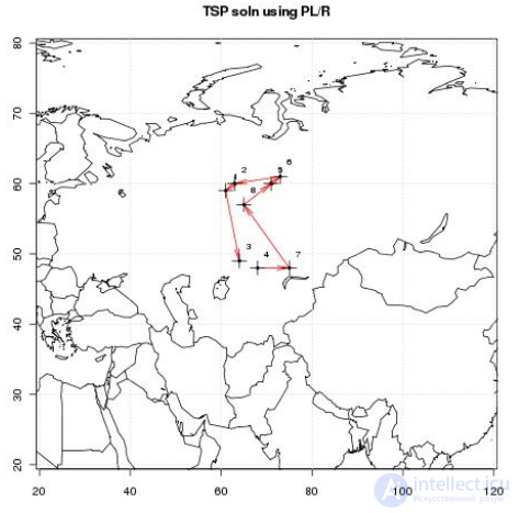
 INSERT INTO plr_modules VALUES ( 1, $$make.map <-function(tour, waypts, mapname) { require(maps) jpeg(file=mapname, width = 480, height = 480, pointsize = 10, quality = 75) map('world2', xlim = c(20, 120), ylim=c(20,80) ) map.axes() grid() arrows( waypts[tour[1:(length(tour)-1)],]$x, waypts[tour[1:(length(tour)-1)],]$y, waypts[tour[2:(length(tour))],]$x, waypts[tour[2:(length(tour))],]$y, angle=10, lwd=1, length=.15, col="red" ) points( waypts$x, waypts$y, pch=3, cex=2 ) points( waypts$x, waypts$y, pch=20, cex=0.8 ) text( waypts$x+2, waypts$y+2, as.character( waypts$id ), cex=0.8 ) title( "TSP soln using PL/R" ) dev.off() }$$ ); 

We start the function of receiving TSP tags:

 -- only needed if INSERT INTO plr_modules was in same session SELECT reload_plr_modules(); SELECT seqid, plotid, bearing, distance, velocity, traveltime, loitertime, totaltraveldist FROM solve_tsp(true, 'tsp.jpg'); NOTICE: tour.dist= 2804.58129355858 seqid | plotid | bearing | distance | velocity | traveltime | loitertime | totaltraveldist -------+--------+---------+----------+----------+------------+------------+----------------- 1 | 8 | 131.987 | 747.219 | 500 | 1.49444 | 0.5 | 747.219 2 | 7 | -90 | 322.719 | 500 | 0.645437 | 0.5 | 1069.94 3 | 4 | 284.036 | 195.219 | 500 | 0.390438 | 0.5 | 1265.16 4 | 3 | 343.301 | 699.683 | 500 | 1.39937 | 0.5 | 1964.84 5 | 1 | 63.4349 | 98.2015 | 500 | 0.196403 | 0.5 | 2063.04 6 | 2 | 84.2894 | 345.957 | 500 | 0.691915 | 0.5 | 2409 7 | 6 | 243.435 | 96.7281 | 500 | 0.193456 | 0.5 | 2505.73 8 | 5 | 0 | 298.855 | 500 | 0.59771 | 0.5 | 2804.58 (8 rows) 

Advanced view:

 \x SELECT * FROM solve_tsp(true, 'tsp.jpg'); NOTICE: tour.dist= 2804.58129355858 -[ RECORD 1 ]---+--------------------------------------------------- seqid | 1 plotid | 3 bearing | 104.036 distance | 195.219 velocity | 500 traveltime | 0.390438 loitertime | 0.5 totaltraveldist | 195.219 totaltraveltime | 0.890438 location | 0101000020E610000000000000000050400000000000804840 -[ RECORD 2 ]---+--------------------------------------------------- [...] 

Thus, we got the order in which it is worth visiting these cities, the distance between them, etc. In addition, we have a visual solution to the traveling salesman problem:


Consider another example, this time with seismic data.

When an earthquake occurs, it usually lasts 15-20 seconds, and seismologists collect data on the intensity of its vibrations. That is, we have time series (timeseries) of data in a waveform data format. Data is stored as an array of floating-point numbers (floats) recorded during a seismic event with a constant sampling rate. They are available from online sources in separate files for each activity. Each file contains about 16,000 items.

Download 1000 seismic activities using PL / pgSQL:

 DROP TABLE IF EXISTS test_ts; CREATE TABLE test_ts ( dataid bigint NOT NULL PRIMARY KEY, data double precision[] ); CREATE OR REPLACE FUNCTION load_test(int) RETURNS text AS $$ DECLARE i int; arr text; sql text; BEGIN arr := pg_read_file('array-data.csv', 0, 500000); FOR i IN 1..$1 LOOP sql := $i$INSERT INTO test_ts(dataid,data) VALUES ($i$ || i || $i$,'{$i$ || arr || $i$}')$i$; EXECUTE sql; END LOOP; RETURN 'OK'; END; $$ LANGUAGE plpgsql; SELECT load_test(1000); load_test ----------- OK (1 row) Time: 37336.539 ms 

This can be done differently, with the help of R, and it will take two times less time - the rare case when using PL / R speeds up, rather than slows down the process:

 DROP TABLE IF EXISTS test_ts_obj; CREATE TABLE test_ts_obj ( dataid serial PRIMARY KEY, data bytea ); CREATE OR REPLACE FUNCTION make_r_object(fname text) RETURNS bytea AS $$ myvar<-scan(fname,sep=",") return(myvar); $$ LANGUAGE 'plr' IMMUTABLE; INSERT INTO test_ts_obj (data) SELECT make_r_object('array-data.csv') FROM generate_series(1,1000); INSERT 0 1000 Time: 12166.137 ms 

Create an oscillogram:

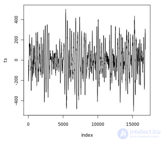
 CREATE OR REPLACE FUNCTION plot_ts(ts double precision[]) RETURNS bytea AS $$ library(quantmod) library(cairoDevice) library(RGtk2) pixmap <- gdkPixmapNew(w=500, h=500, depth=24) asCairoDevice(pixmap) plot(ts,type="l") plot_pixbuf <- gdkPixbufGetFromDrawable( NULL, pixmap, pixmap$getColormap(), 0, 0, 0, 0, 500, 500 ) buffer <- gdkPixbufSaveToBufferv( plot_pixbuf, "jpeg", character(0), character(0) )$buffer return(buffer) $$ LANGUAGE 'plr' IMMUTABLE; SELECT plr_get_raw(plot_ts(data)) FROM test_ts WHERE dataid = 42; 

We get this picture for a specific earthquake:


Now it needs to be analyzed in order, for example, to find out how best to design buildings in an area with similar seismic activity. You probably remember from the school physics course such a thing as "resonant frequency." Just in case, let me remind you that this is such an oscillation frequency at which the amplitude of oscillations increases sharply. This frequency is determined by the properties of the system. That is, in a zone with seismic activity, it is necessary to design buildings in such a way that their resonant frequency does not coincide with the frequency of earthquakes. This can be done with R:

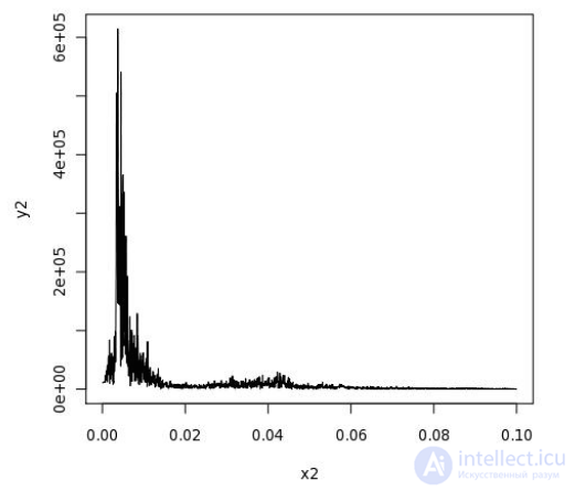
 CREATE OR REPLACE FUNCTION plot_fftps(ts bytea) RETURNS bytea AS $$ library(quantmod) library(cairoDevice) library(RGtk2) fourier<-fft(ts) magnitude<-Mod(fourier) y2 <- magnitude[1:(length(magnitude)/10)] x2 <- 1:length(y2)/length(magnitude) mydf <- data.frame(x2,y2) pixmap <- gdkPixmapNew(w=500, h=500, depth=24) asCairoDevice(pixmap) plot(mydf,type="l") plot_pixbuf <- gdkPixbufGetFromDrawable( NULL, pixmap, pixmap$getColormap(), 0, 0, 0, 0, 500, 500 ) buffer <- gdkPixbufSaveToBufferv( plot_pixbuf, "jpeg", character(0), character(0) )$buffer return(buffer) $$ LANGUAGE 'plr' IMMUTABLE; SELECT plr_get_raw(plot_fftps(data)) FROM test_ts_obj WHERE dataid = 42; 

And this is how the final result looks like, showing the frequency of vibrations and their amplitude:


Having such a schedule before his eyes, the architect can make calculations and design a structure that does not collapse at the very first quake.

As you can see, PL / R has many uses, as it allows you to link advanced analytics to databases and at the same time use the functionality of R and PostgreSQL with all their advantages. I hope this article will be useful to you, and you will find the use of such an effective and multifunctional tool.