Lecture
Basic definitions
The functioning of many IP is focused. A typical act of such functioning is to solve the problem of planning the way to achieve the desired goal from a fixed initial situation. The result of solving the problem should be an action plan - a partially-ordered set of actions. Such a plan resembles a scenario in which the relations between the vertices are relations of the following type: “goal-subgoal”, “goal-action”, “action-result”, etc. Any way in this scenario that leads from the vertex corresponding to The current situation, in any of the target vertices, determines the action plan.
The search for an action plan arises in the IP only when it encounters a non-standard situation for which there is no known set of actions leading to the desired goal. All tasks of building an action plan can be divided into two types, which correspond to different models: planning in the state space (SS-problem) and planning in the task space (PR-problem).
In the first case, a certain situation space is considered to be given. The description of situations includes the state of the outside world and the state of IP, characterized by a number of parameters. Situations form some generalized states, and actions of IP or changes in the external environment lead to a change in the actualized states at a given moment. Among the generalized states, the initial states (usually one) and the final (target) states are distinguished. The SS-problem consists in finding a path leading from the initial state to one of the final ones. If, for example, the IC is designed for playing chess, then the generalized states will be the positions that are formed on the chessboard. The position that is fixed at the moment of the game can be considered as the initial state, and the set of draw positions as the target positions. Note that in the case of chess, a direct listing of target positions is not possible. Matte and draw positions are described in a language different from the language of description of states, characterized by the location of the figures in the margins of the board. That is what makes it difficult to find a plan of action in a chess game.
When planning in the task space, the situation is somewhat different. The space is formed as a result of introducing the following relations on a set of tasks: "part - whole", "task - subtask", "general case - special case", etc. In other words, the task space reflects the decomposition of tasks into subtasks (goals for subgoals) . The PR problem consists in finding the decomposition of the original problem into subtasks leading to the problems that the system knows about. For example, the IC knows how the values of sin x and cos x are calculated for any value of the argument and how the division operation is performed. If the IP needs to calculate tg x, then the solution to the PR problem will be to present this task as a decomposition tgx = a = sinx / cosx (except for l: = l / 2 + k l).
We give a classification of the methods used in solving SS-and PR-problems.
1. Planning by state. The representation of tasks in the state space involves the assignment of a number of descriptions: states, a set of operators and their effects on state transitions, target states. State descriptions can be character strings, vectors, two-dimensional arrays, trees, lists, etc. Operators translate one state into another. Sometimes they are represented as products A => B, meaning that state A is transformed into state B.
The state space can be represented as a graph whose vertices are labeled with states, and arcs with operators. If some arc is directed from the vertex n i , to the vertex n, then n is called a child, and n j ; - parent vertices
The sequence of vertices n i1 , n i2 , ..., n ik , in which each n i -sub-vertex for n ij-1 , / = 2, ..., k, is called a path of length k from the vertex n i1 , to vertex n ik .
Thus, the problem of finding a solution to the problem <A, B> when planning by state is presented as a problem of searching the path graph from A to B. Usually, the graphs are not specified, but are generated as needed.
Blind and directional search methods differ . The blind method has two types: search in depth and search in breadth. When searching deep into each alternative is investigated to the end, without taking into account other alternatives. The method is bad for "tall" trees, because you can easily slip past the desired branch and spend a lot of effort on researching "empty" alternatives. When searching in breadth at a fixed level, all alternatives are investigated and only after that the transition to the next level is carried out. The method may be worse than the search method inland if all the paths leading to the target vertex in the graph are located at about the same depth. Both blind methods are time consuming and therefore targeted search methods are needed.
The method of branches and boundaries. Of the unfinished paths formed in the search process, the shortest path is selected and extended by one step. The resulting new unfinished paths (there are as many as the branches at a given vertex) are considered along with the old ones, and again the shortest one is extended by one step. The process is repeated until the first achievement of the target vertex, the decision is remembered. Then, from the remaining unfinished paths, longer or longer than the completed path are excluded, and the rest are extended by the same algorithm until their length is less than the completed path. As a result, either all unfinished paths are excluded, or among them a complete path is formed, shorter than previously obtained. The last path begins to play the role of the standard, and so on.
Moore's shortest path algorithm. The initial vertex x 0 is marked with the number 0. Suppose that during the operation of the algorithm at the current step, a set of child vertices Γ (x i ) of vertices x i is obtained . Then all previously obtained vertices are deleted from it, the remaining ones are marked with a label increased by one compared to the vertex x i , and pointers to x i are drawn from them . Further, on the set of labeled vertices that do not yet appear as pointers, a vertex with the smallest label is selected and child vertices are constructed for it. The vertex markup is repeated until a target vertex is obtained.
Dijkstra ’s minimum-cost path definition algorithm is a generalization of Moore’s algorithm by introducing arcs of variable length.
Doran and Michie search algorithm with low cost. Used when the search cost is high compared to the cost of the optimal solution. In this case, instead of selecting the vertices that are the least distant from the beginning, as in Moore’s and Dijkstra’s algorithms, a vertex is chosen for which the heuristic estimate of the distance to the target is the smallest. With a good estimate, you can quickly get a solution, but there is no guarantee that the path will be minimal.
Algorithm of Hart, Nilson and Raphael. The algorithm combines both criteria: the cost of the path to the vertex g (x) and the cost of the path from the vertex h (x) are in the additive estimate function f (x) = g (x) + h (x). Under the condition h (x) <h p (x), where h p (x) is the actual distance to the target, the algorithm guarantees finding the optimal path.
Path finding algorithms on the graph also differ in the direction of the search. There are direct, inverse, and bidirectional search methods. Direct search comes from the source state and, as a rule, is used when the target state is implicitly specified. Reverse search comes from the target state and is used when the initial state is specified implicitly, and the target state is explicit. Bidirectional search requires a satisfactory solution to two problems: changing the direction of search and optimizing the “meeting point”. One of the criteria for solving the first problem is to compare the “width” of the search in both directions — the direction that narrows the search is chosen. The second problem is caused by the fact that the forward and reverse paths can diverge and the narrower the search, the more likely it is.
2. Planning for tasks. This method leads to good results because often problem solving has a hierarchical structure. However, it is not necessary to require that the main task and all its subtasks be solved by the same methods. The reduction is useful for representing the global aspects of the problem, and for solving more specific problems, the state planning method is preferable. The state planning method can be considered as a special case of the planning method using reductions, because each application of an operator in the state space means reducing the initial problem to two simpler ones, one of which is elementary. In the general case, the reduction of the original problem does not reduce to the formation of such two subtasks, of which at least one was elementary.
The search for planning in the task space consists in the sequential reduction of the initial task to an ever more simple one until only elementary tasks are received. A partially ordered set of such tasks will make up the solution to the original problem. The division of the problem into alternative sets of subtasks is conveniently represented in the form of an AND / OR graph. In such a graph, each vertex, except the terminal, has either conjunctively connected child vertices (AND-vertex) or disjunctively connected (OR-vertex). In the particular case, in the absence of I-vertices, there is a graph of the state space. Terminal vertices are either final (they correspond to elementary problems) or dead-end. The initial vertex (root of an AND / OR graph) represents the original problem. The purpose of the search on an AND / OR graph is to show that the initial vertex is solvable. The solvable are final vertices (AND-vertices), in which all child vertices are solvable, and OR-vertices, in which at least one child vertex is solvable. The resolving graph consists of solvable vertices and indicates the solvability method of the initial vertex. The presence of dead-end vertices leads to unsolvable vertices. Dead-end vertices are unsolvable, AND-vertices for which at least one daughter vertex is insoluble, and OR-vertices for which each daughter vertex is unsolvable.
Algorithm of Cheng and Slaig. It is based on the transformation of an arbitrary AND / OR-graph into a special OR-graph, each OR-branch of which has AND-vertices only at the end. The transformation uses the representation of an arbitrary AND / OR graph as an arbitrary formula of propositional logic with a further transformation of this arbitrary formula into a disjunctive normal form. Such a transformation allows you to further use the algorithm of Hart, Nielson and Raphael.
Key operator method. Let the task <A, B> be given and it is known that the operator f must necessarily be included in the solution of this problem. Such an operator is called key. Suppose that for the application of f a state C is necessary , and the result of its application is f (c). Then the I-vertex <A, B> generates three child vertices: <A, C>, <C, f (c}> and <f (c), B>, of which the average is an elementary task. To the problems <A, C> and <f (c), B> key operators are also selected, and this reduction procedure is repeated as long as possible. As a result, the initial task <A, B> is divided into an ordered set of subtasks, each of which is solved by the planning method in the state space.
Alternatives are possible at the choice of key operators, so in the general case the AND / OR graph will take place. In most of the tasks, it is possible not to single out the key operator, but only to indicate the set containing it. In this case, for the task <A, B>, the difference between A and B is calculated , to which the operator is correlated, which eliminates this difference. The latter is the key.
The method of planning a common problem solver (ORZ). ORZ was the first most famous planner model. It was used to solve problems of integral calculus, inference, grammatical analysis, and others. The ORZ unites two basic principles of search:
analysis of goals and means and recursive problem solving. In each search cycle, the ORZ decides in a rigid sequence three types of standard tasks: convert object A to object B, reduce the difference D between A and B, apply operator f to object A. The solution of the first problem determines the difference D of the second — the appropriate operator f, and the third — the required condition for the application of C. If C is not different from A, then the operator f is applied, otherwise C is presented as another goal and the cycle repeats, starting with the task "convert A to C". In general, the strategy of ORZ performs a reverse search - from a given goal B to the required means of achieving it C, using the reduction of the original task <A, B> to the tasks <A, C> and <C, B>.
Note that in the ORZ it is tacitly assumed independence of differences from each other, whence follows the guarantee that the reduction of some differences will not lead to an increase in others.
3. Planning with inference. Such planning assumes: the description of states in the form of correctly constructed formulas (PPF) of some logical calculus, the description of operators in the form of either PPF, or the rules for transferring some PPF to others. Representation of operators in the form of PPF allows you to create deductive planning methods, the representation of operators in the form of translation rules - planning methods with elements of deductive inference.
The deductive method of planning the system QA3 , ORZ did not justify the hopes placed on it mainly due to the unsatisfactory presentation of the tasks. An attempt to rectify the situation led to the creation of a QA3 question-answer system. The system is designed for an arbitrary subject area and is able, by inference, to answer the question: is it possible to achieve state B from A? The resolution principle is used as a method of automatic withdrawal. For the direction of logical inference, QA3 applies various strategies, mainly of a syntactic nature, taking into account the peculiarities of the formalism of the principle of resolutions. Operation QA3 showed that the output in such a system is slow, detailed, which is not typical of human reasoning.
STRIPS production method . In this method, the operator represents the products P, A => B, where P, A, and B are sets of FFTs of the first order predicate calculus, P expresses the conditions for using the production core A => B, where B contains the list of added FPS and the list of excluded FFTs . e. postconditions. The method repeats the ORZ method with the difference that the standard tasks of determining differences and applying suitable operators are solved on the basis of the principle of resolutions. Approaching The main operator is selected in the same way as in the ORZ, on the basis of the principle “analysis of means and goals”. The presence of a combined planning method made it possible to limit the process of logical inference to a description of the state of the world, and leave the process of generating new such descriptions to the heuristics “from the goal to the means to achieve it”.
Method of production using macro operators . Macro operators are generalized solutions to problems obtained by the STRIPS method. The use of macro-operators allows reducing the search for a solution; however, this raises the problem of simplifying the applied macro-operator, the essence of which lies in identifying its required part for a given difference and excluding unnecessary operators from the latter.
ABSTRIPS solver hierarchical production method. In this method, the partitioning of the search space into hierarchy levels is performed using the detailing of the products used in the STRIPS method. To do this, each LPS of the PPS, which is included in the set P of the conditions of use of the products, is assigned a weight j, j = 0, k, and at the i-th level of planning, carried out by the STRIPS method, only letters of weight j are taken into account . Thus, at the k-th level of production are described in the least detail, at zero — the most detailed as in the STRIPS method. Such a partition allows for planning at the jth level to use the (j + 1) -th level solution as the skeleton of the jth level solution, which increases the efficiency of the search as a whole.
An improved method of planning Newell and Simon. The method is based on the following idea of further improving the ORZ method: the problem is solved first in the simplified (due to the ranking of differences) planning area, and then an attempt is made to clarify the solution for a more detailed, original problem area.
Complex fuzzy planning scheme
The disadvantage of the majority of currently known planning systems is their rigid binding to the planning scheme. Any of them is always looking for a solution to either SS-problems or PR-problems. This is due to the fixation of the presentation of information for planning. For the classic models of SS- and PR-problems, these forms are different. It is clear, however, that a person successfully combines the planning steps of solving SS- and PR-problems in his activity. The second disadvantage is the determination of planning systems. In real IS, determinism of planning, as a rule, does not take place. The generalization of fuzzy SS and PR problems consists in the assumption of fuzzy states and fuzzy operators of the transition from state to state. The division of the problem into subtasks has weights on arcs with values from [0, 1], which are interpreted as the reliability of the solution of the corresponding subproblems. The reliability of a solution to a PR problem is determined by at least the reliability of a solution to its sub-problems.
In the transition to a generalized strategy, from solutions of fuzzy subproblems of the PR problem, considered as fuzzy SS problems, one can get a solution of the fuzzy PR problem, also considered as a fuzzy SS problem.
The SS-problem scheme is the pair M = (S, G), where S is the set of states, G is the set of mappings g: S-> S, called operators. The path from the state s 0 eS to the state s r eS is called the final sequence p = ((s 0 ,, g 0 ), ( s 1 , g 1 ), ..., ( s k-1 , g k-1 ) s k ) , such that g i O s i = s i + 1 for 0, ..., k- 1. The SS-problem is the quadruple P = (S, G, i, f), where (S, G ) - SS-problem circuit, i, fеS-initial and final state, respectively. The path x, leading from i to f, is a solution to P, and the set of all such paths constitutes a set of solutions.
The scheme of a PR problem is the pair .N = ( S , Γ), where S is the set of problems, and Γ is the set of mappings g : S -> S + , called operators. If Re S , p e S + , then g p ( p ) is a map representing the problem P in the form of a chain of subproblems p = P1 ... Pn. For the scheme N = ( S , Γ), covering the path q from the problem s 0 to a finite set of problems S k = { s 1 , ..., s }} e S | is a finite sequence, where q = (( x 0 , y 0 ), ( x 1 , y 1 ), ..., ( x k-1 , y k-1 ), x k ), x i e S + for i = 0, ..., k, yEG + for i = 0, ..., k-1, so that x 0 = s 0 , x k e S + k . PR-problem is a quadruple Z = ( S , G, Ro, F), where ( S , G) is a scheme of PR-problems, R o e S is the initial problem, F M S is the set of final problems. The solution Z is the covering path ( S , Γ) from P o to F / x; M Φ, the set of solutions x z , is the set of all solutions of Z.
The above definitions consider only the syntax of the problem description, regardless of the meaning of the formal scheme used. In the SS-problem scheme, the syntax and semantics may coincide in more complex cases, for example, in the PR-problem scheme, they should differ. By semantics, here we mean the way in which the solution of the problem sought is obtained from the solutions of the subtasks to which it has been reduced. We give a formal definition of the semantics of reducing a problem to subtasks.
The implicate of problem P is a pair ( p , y ), where p = P i P 2 ... P k is a chain of problems, y is a mapping from X p1 C X p2 ... C X pk to X p ( X pi means
the set of solutions P i <). An implicative scheme is a triple L = (P, p , y ), such that P is a problem, ( p , y ) is an implicate R. A set T of implicative schemes is called an implicative network. Many problems of implicative network
W t = {x | ( $ L ) (( L = (P, p , y ) ) L ((x = P) \ / (x is a symbol p ))}.
Let us combine the syntax and semantics of the approach based on breaking the problem into subproblems. PR-проблема Z=( S , Г, Ро, Ф) представляет импликативную сеть Т тогда и только тогда, когда S = W t и для каждого L =(Р, p , y )эT существует в точности одно g эГ, такое, что Р g = p , и для каждого g эГ, и для каждого Р из области определения g существует в точности одно L =(Р, p , Y ) ' T, такое,что p =P g Проблема Р решена тогда и только тогда, когда Х p - непустое множество.
Если PR-проблема представляет импликативную сеть, то проблема Р 0 разрешима. Для существования решения достаточно, чтобы импликативные схемы в импликативной сети Т существовали только для всех пар (xi, у,), i=0,..., k- 1, входящих в накрывающий путь схемы PR-проблемы. В этом случае синтаксис и семантика PR-проблемы не совпадают. В данном случае PR-проблема частично представляет импликативную сеть Т.
Подчеркнем, что как синтаксис, так и семантика подхода разбиения проблемы на подпроблемы не предполагают предварительного определения проблемы. Поэтому можно в качестве проблемы выбрать SS-проблему.
Consider a concept that combines approaches for splitting a problem into sub-problems and searching in the state space. The 1-problem (the combined problem) is the quadruple R = (B, G, P 0 , T), where B is the set of SS problems;
(В, Г)-схема PR-проблем; Р 0 эB -основная проблема;T-импликативная сеть, такая, что W T З B © Ж . Кроме того, R есть решение SS-проблемы Р 0 . Учитывая связь между существованием импликативной сети и разрешимостью проблемы, легко показать, что если для заданной I-проблемы найден накрывающий путь х из Р 0 на множество Ф' Н В, проблемы Ф' разрешимы как SS-проблемы, если х частично представляет импликативную сеть Т, то и проблема R разрешима как SS-проблема.
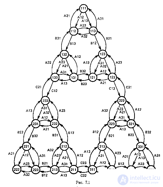
Рассмотрим головоломку "Ханойская башня" . Имеются три стержня 1, 2 и 3 и три диска различных размеров А, В, С с отверстием в центре, которые могут одеваться на стержни. В исходной позиции диски находятся на стержне 1; самый большой диск С-внизу, самый маленький диск А- наверху. Требуется перенести все диски на стержень 3, перемещая за один раз только один диск. Брать можно только самый верхний диск на стержне, причем его нельзя класть на диск, меньший по размерам. Используем для записи состояний и операторов классическую формализацию. Выражение ijk обозначает конфигурацию, при которой диск С находится на стержне i, диск В - на стержне j и диск А-на стержне k. Выражение xij обозначает действие, при котором диск х перемещается со стержня i на стержень j. С помощью этого формализма можно просто записать все состояния и переходы головоломки в виде треугольного графа, где вершины соответствуют расположению дисков на стержнях, а дуги-возможным перекладываниям дисков (рис.1). На этой головоломке легко проиллюстрировать все основные понятия обобщенной стратегии проблем.
Представим головоломку в виде модели I-проблемы. Рассмотрим I-проблему R=(B, Г, P 0 T), где B={Р 0 , P 1 ,...,P 9 }; Г={ g }; T=={ L 1 , L 2 , L 3 }. SS-проблемы Р 0 ,P 1..., P 9 определяются следующим образом. In fig. 1 показана схема SS-проблемы M==(S, G), где
P 0 =(S, G, 111, 333), P 1 =(S, G, 111, 122), P 2 =(S, G, 122, 322),
Рз=(S, G, 322, 333), P 4 =(S, G, 111, 113), P 5 ,=(S, G, 113, 123),
P 6 ==(S, G, 123, 122), P 7 =(S, G, 322, 321), P 8 =(S, G, 321, 331),
P 9 =(SG, 331,333).
Схема PR-проблемы N= (В, Г) приведена на рис. 2; импликативная сеть Т - на рис.3, причем L 1 =(P 0 , P 1 Р 2 Р 3 , Y ), L 2 = (P 1 , P 4 P 5 P 6 , Y ), L з== (Р 3 , P 7 P 8 P 9 , Y ), где Y (x 1 ,x 2 ,x 3 )=x 1 x 2 x 3 .
Проблемы Р 2 и P 4 -P 9 решаются перекладыванием одного диска и являются элементарными. Проблемы P 1 и Р 3 решаются с помощью манипуляций только с дисками В и А и являются более простыми, чем Р 0 . Проблемы P 1 и Р 3 решаются, а проблема Р 0 сводится к P 1 , P 2 и Р 3 аналогичной манипуляцией с дисками, синтаксис которой выражен оператором g , а семантика - отображением Y .
Представление этой головоломки в виде PR-проблемы (рис.2) является более компактным и наглядным, чем представление в виде SS-проблемы (рис.1), а представление в виде I-проблемы (рис..3) сочетает достоинство обоих и показывает взаимосвязь подпроблем и тех действий, которые нужно выполнить, чтобы решить головоломку.
Приведенные определения обобщаются на нечеткий случай, когда состояние системы, для которой строится модель решения проблемы, не является точно заданным, а результаты действий системы
неоднозначны.
Например,у робототехнической системы это может быть связано с несовершенством эф-фекторов и рецепторов, с ограниченными размерами внутренней модели, не отражающей сложности окружающего мира.
Нечеткой SS-проблемой назовем SS-проблему, у которой i , f- нечеткие множества, операторы g эG-нечеткие матрицы, a -решением нечеткой SS-проблемы называется путь g=g 1 ...g n ,g i эG,i=1,...,n, такой, что iOg 1 O ... ... Og n Of ? a , где О - максимальное произведение нечетких матриц.
Нечеткой PR-проблемой называется PR-проблема, у которой элементам g эГ приписывается степень принадлежности m g ( p )э[ 0,1], a -решением нечеткой PR-проблемы называется решение PR-проблемы, для которой min g ij ? a , g ij эy i .

Накрывающий путь в этом случае называется накрывающим a -путем. Степень принадлежности m g ( p ) интерпретируется как степень возможности разбиения проблемы на подпроблемы.
Нечеткой импликативной схемой называется импликативная схема, все отображения Y которой имеют степень принадлежности m Y ( ( p )э[0,1]. Степень принадлежности интерпретируется как возможность получения решения проблемы из решений соответствующих подпроблем. Нечеткой импликативной сетью называется импликативная сеть с нечеткими импликативными схемами.Нечеткая PR-проблема представляет нечеткую импликативную сеть, если кроме обычных условий для импликативной сети выполняется неравенство m Y ( p ) ? m g ( p ) ? a ,
т. е. возможность разбиения на подпроблемы не меньше возможности получения решения для каждой пары соответствующих Y и g .
Аналогично определяется нечеткая I-проблема. Но построить a -решение нечеткой PR-проблемы по a -решениям ее нечетких подпроблем можно лишь в частных случаях и при наложении дополнительных условий. Пусть задана нечеткая PR-проблема, где S -нечеткие SS-проблемы, и существует простейшее a -решение Z,
i.e. such p e S + , what is m g p ? a , and if p = P 1 ..P n , then all problems P i are a -solvable,
where Pi = (Si, Gi, Ji, Fi ). a solution to the problem P 0 exists when m Y ( p ) ? m g ( p ) ? a for an implicative network. Let us write a more constructive condition for this. Let for all i the operator g i be the a -path to solve the problem P i and F i = J i + 1. Then, if
max m [F n З (F n-1 З (... F 1 З (J og 1 ) og 2 ) ...) og n )] ? a
and g = g 1 ... g n , then g- a is a solution to the SS problem P 0 .
Features planning targeted actions
Further development of the theory of planning was associated with the construction of "human" models of purposeful activity. If we present human reasoning related to planning as some purposeful activity on solving intellectual problems, then the planning model first of all needs to take into account the main features of human reasoning.
Let some objective world be given in which the action of the IC is to achieve the target situations s k from some initial situations s n using action plans; V = bi1 ... b in , where the bi-executive module is from the given set B 0 . To set a situation s in such a world is to indicate the properties with i О С of objects a k О A 0 and the relations between them r p О R 0 that had, have or will take place at time t. A model of the objective world for such an action of an IS can be represented as Mo = <Ao, Bo, Co, Ro>, and the task of planning actions in the Mo world as follows: the initial s n and target s k "situations are set, it is necessary to build from the executive modules b i О In plan of action V, which, being applied to Sn, allows to reach Sk.
Before a person in solving this problem usually arise two problems. Firstly, it, as a rule, poorly represents a specific s k , remote in the future. Therefore, he is satisfied with the achievement not of a specific, but of any situation from the class s k , which satisfies certain requirements. Secondly, even if it represents s k , then even the search for a plan of action is difficult because of the large dimension of the search space. So, IPs need more general models of Mo in relation to Mo.
Among the tasks we select the elementary class. The rest will be considered complex, and their solutions should be presented in the form of a partially ordered set of elementary tasks. If the solutions to various complex problems are in some sense similar, then they are generalized. So there are generalized descriptions of tasks of a certain type.
From the solutions of elementary problems, the IP builds solutions to complex initial problems. However, she did not usually find a solution in this way immediately. Therefore, typical problems are used to move from initial to elementary tasks. First, for the given initial task, the semantic structure of its initial data is determined, that is, a strategic task is set and its solution hypothesis is formed. Further, each typical problem of the hypothesis is decomposed, which leads to the formulation and solution of tactical problems and, consequently, to the solution of the original problem.
The presence in the knowledge base of typical and elementary tasks testifies to the hierarchical structure of not only the knowledge base, but also search procedures, while typical tasks can be conditionally assigned to the strategic and elementary tasks to the tactical level of the search. The semantic structures of the required results and initial data of typical tasks are usually revealed as a result of comprehension of the required results or initial data of tactical tasks and are not available to direct sensory perception. Thus, at the strategic level, each tactical situation (initial data or the desired result) is evaluated by the presence in it of familiar semantic structures. For example, in a chess game, semantic structures are expressed by the notion “developed position”, “open position”, etc. At the tactical level, tactical tasks projected from a strategic level are solved by decomposing typical tasks, such as the formation of a passed pawn in a chess game.
So, the basis of the EC reasoning on action planning is structured knowledge and directed heuristic search.
Let C 1 be the set obtained by coarsening the properties with O C 0 , B 1 the set of elementary problems obtained by renaming the execution modules b i O B 0 , A 1 ≤ A and R 1 ≤ Ro. Then the model of the world of tactical tasks can be represented as Mo = <A 1, B 1, C 1, R 1>, the formulation of the tactical task p-
in the form of a pair <s n , s k >, and its solution in the form of a set V = L 1 , ..., b in . Obviously, due to this coarsening in the world of M 1 , separate states of objects and executive modules become indistinguishable. However, such a simplification, caused by the "rudeness" of the senses of the IP, still does not significantly reduce the dimension of the solution search space V; therefore, further generalization of M 1 is needed at the conceptual level.
In the world M 1, tactical situations s are described, as well as situations s in the world M 0 , through the properties of objects and the relations between them. However, such descriptions are not holistic in nature, since they do not explicitly contain semantic structures. The identification of such generalized structures, as well as the formation of the corresponding tactical situations s, are carried out on the basis of the concepts possessed by the information system, and they mean comprehending existing or target situations s from the point of view of these concepts used in this case as test programs. Thus, in the world M 2, the indicated situations are represented as enlarged objects a k О A 2 , the properties of which c i О C 2 and the relations r 2 О R 2 between which, like the enlarged objects themselves, are determined by the concepts-tests. The situation is similar with solutions V in the world M 1 . Holistic description of V means the description of these solutions as typical problems. Thus, in the world M 2 there are typical tasks b i О B 2 .
Estimates of the complexity of the planning task
We present a number of results concerning the complexity of solving planning problems.
1. Analysis of computational problems turns out to be a PSPACE-complete problem, even if there are no “empty” values of W.
2. For computational models without functional quantities, i.e., with empty D b and F, the problem of analyzing computational problems turns out to be: a) PSPACE-complete for H containing functional and operator dependencies without W ; b) NP-complete for H, containing only functional and variant dependences without the “empty” value W ; c) polynomial (according to the scheduler operation time) for H, containing only functional and implicit dependencies; d) it is possible to construct planners with linear operation time for H only with functional dependencies without W and for H with functional and implicit dependencies.
In the PGIZ system, D b and F are empty, and in H there are only functional and operator dependencies without the “empty” values of W. The system of automatic synthesis of programs SPORA uses predicate calculus, for which a special inference strategy has been developed.
An analysis tree for a computational problem is a tree of formulas used in calculus, at the root of which is a formula representing the original problem, each non-terminal vertex of the tree can be obtained by one of the rules for deriving a “calculus of computational problems” from formulas located in the tree directly below, and terminal (pendant) vertices are not the conclusion of any of the rules for deriving "calculus of computational problems".
The scheduler in this calculus works as follows: for a given task, some analysis tree is constructed. If all its pendant vertices are axioms, then a program is assembled along this tree. Otherwise, a justification is formed that the task is unsolvable. The absence of determinism in logical inference in calculus of the standard type leads to an exponential sorting out of possible branches. Detection with this enumeration of the impasse turns out to be useless (or almost useless) for searching other branches of the output tree. In the "calculus of computational problems" for a complete solution of the problem, the planner is sufficient to have some kind of analysis tree. With a reasonable strategy for building analysis trees, this allows for relatively quick planning procedures.
In general, the scheduler has to solve a PSPACE-complete task. This means that all currently known planners run exponential time on almost all computational problems. In reality, the situation is not so bad. Practically interesting tasks, as a rule, allow effective planning. And although the proportion of such tasks with an increase in the parameters defining them, tends to zero, they are of interest from the point of view of the efficiency of automatic program synthesis. An indicator of practically interesting problems can be the degree of interaction of subtasks in the process of solving the original problem. The concepts of "subtask" and "conditions of subtasks" arise already at the stage of a naive interpretation of the following dependencies.
Functional dependencies (F-> Y 1 ), where F is a functional value of the type (X -> - Y), which assumes a preliminary synthesis of the procedure for calculating F, the input parameters of which are the values from the list X.
Operator dependencies involving the synthesis of t procedures with inputs "subtask conditions" X 1 , X 2 , ..., X b -
Variant dependencies that assume that two branches of calculations are created: for the first one, the values of all the quantities from the list Y 1 are known , and for the second, from the list Y 2 .
Consider a simple (but typical) example. Let there be a functional dependence D 1 : (A, B, C R E) and operator dependencies D 2 : (( С R Е ) R Е 1 ), D 3 : ((B R Е 1 ) ) R Е 2 )) , D 4 : (( A R E 2 ) R E 3 ) . Need to find Ez. To do this, solve the subtask ( A R E 2 ) . If we use the dependence D 3 , we come to the search for a solution to the new subtask (B R E 1 ). If we use the dependence D 2 , we come to the necessity of solving the subtask (C R E), which, according to D 1, is solvable only when A and B are known. The degree of interaction of subtasks in this example is three. A process is a typical task space planning scheme.
For planners working in the "calculus of computational problems;", the synthesis of solving a computational problem occurs during the time hq r l / r !, where h is a constant, l is the length of the task record, defined as the total number of occurrences of the names of the values used in F and H, q is the total number of “different” arguments of the quantities from the “subtask condition” in the operator dependencies from H and the “variant conditions” in the variant dependencies from H, r is the minimum degree of interaction between the subtasks in the original problem. This estimate is quasi-optimal. The scheduler works for a long time only on those tasks that are not natural, since they require that all the subtasks into which the original task is interlaced are bound together. Experiments show that for tasks encountered in practice, the work time of the scheduler is polynomial. The memory necessary for the work of the scheduler in the "calculus of computational problems" is estimated to be bl 2 , where b is a constant. If there are no variant dependencies in H , then linear memory size dl is required , where d is a constant.
In currently known planners, the programs obtained are far from optimal. There is a tendency of deterioration in the quality of programs with a decrease in the time of the scheduler. At the same time, it is more difficult to synthesize optimal sequential programs than optimal parallel programs. This circumstance in connection with the development of the computer of a new architecture oriented to parallel processes can be profitable. For example, the task of finding the minimum time sequential execution of programs for solving computational problems for which D b is empty, and H consists only of functional dependencies W , turns out to be NP-complete in a strong sense. On the other hand, in the "calculus of computational problems", provided that D b is empty, and H consists of functional and implicit dependencies, it is possible for linear time kl (k - constant) to synthesize a program whose parallel execution requires the minimum time for a given task.
In the PRIZE system and its modifications, the computational problem is considered solvable if the corresponding formula is derivable in the positive fragment of the intuitionistic propositional calculus, that is, if and only if success is achieved by the PRIZER planner. For the "calculus of computational problems" two semantics are possible for solvability.
Extremely unconstructive; A computational problem is considered solvable if in any database (any interpretation) that satisfies all the constraints of the computational model, there is a certain function of the type (X R Y);
extremely constructive: a generalized standard scheme of a program is considered a solution to a computational problem if, in any interpretation that satisfies all the constraints of the computational model, there is a function (X R Y) calculated by program P, obtained from the generalized standard scheme of the program by the corresponding specification of predicate and functional symbols.
The "calculus of computational problems" is correct and complete with respect to both semantics. With the first semantics, the scheduler always gives a solution to the original problem in the form of a regular program, with the second, the class of all propositional formulas describing solvable computational problems coincides with the class of all formulas derived in the intuitionistic propositional calculus. This shows that the “calculus of computational problems” can be viewed as one of the options for formalizing the intuitionistic logic proposed in the interpretation of logic as the logic of “problems”.
In many IS, planners are used, the capabilities of which are significantly wider than those of the PRIZE system scheduler, or that used in the “calculus of computational problems”. The calculi, dealt with by many planners of computer-aided design, planning and management, is broader than intuitionistic calculus of propositions. At the same time, heuristic considerations are used, which have no analogues in the ratios in which the computational models were described. An example would be the scheduler of the system MAVR, intended for IP computer-aided design. When his work there are situations that are not solvable in the theory described above. Such cases force you to look for other ways to build a system to search for action plans.

Comments
To leave a comment
Intelligent Information Systems
Terms: Intelligent Information Systems