Lecture
The idea of a detailed device of the brain appeared only about a hundred years ago. In 1888, Spanish doctor Ramoni Kayal experimentally showed that brain tissue consists of a large number of interconnected homogeneous nodes - neurons. Later studies using an electron microscope showed that all neurons, regardless of type, have a similar organizational structure (Fig. 2.1). The natural nerve cell (neuron) consists of the body (soma) containing the nucleus, and the processes - the dendrites, through which the neuron receives input signals. One of the processes, branching at the end, serves to transmit the output signals of a given neuron to other nerve cells. It is called an axon. The connection of the axon with the dendrite of another neuron is called a synapse. A neuron is excited and transmits a signal through an axon if the number of exciting signals coming through the dendrites is greater than the number of inhibitory signals.
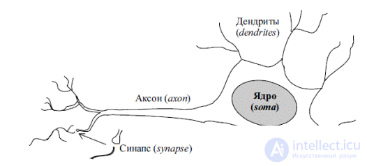
Figure 2.1 - The structure of a biological neuron.
In 1943, V. McCulloch and V. Pitts proposed an information processing system in the form of a network consisting of simple calculators created according to the principle of a biological neuron. An artificial neural network (ANN) is a collection of simple computing elements (processors) - artificial neurons connected in some way so that interaction between them is provided. Artificial neurons are characterized by the rule of combining input signals and the transfer function, allowing to calculate the output signal.
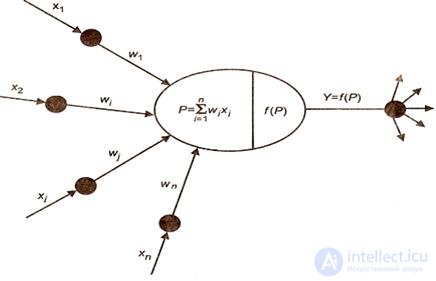
Figure 2.2 - Cybernetic model of a neuron.
Information received at the input of the neuron is summed up taking into account the weighting coefficients of the signals:
 , (2.1)
where w 0 is the shift (threshold, offset) of the neuron.
Depending on the value of the weighting factor w i , the input signal x i is either amplified or suppressed. The weighted sum of the input signals is also called the potential or the combined input of the neuron.
The shift is usually interpreted as a bond emanating from an element whose activity is always 1. Usually, for convenience, the input vector is expanded by adding this signal to x = (1, x 0 , ..., x n ) and the threshold w 0 is entered under the sum sign :
 . (2.2)
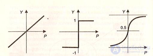
The transfer function, or neuron activation function, is a rule according to which the weighted sum of incoming signals P is converted into the output signal of neuron Y, which is transmitted to other neurons of the network, i.e. Y = f (P). Figure 2.3 shows graphs of the most common neuron activation functions.
The threshold function passes information only if the algebraic sum of the input signals exceeds a certain constant value P *, for example:

The threshold function does not provide sufficient flexibility of the ANN when training. If the value of the calculated potential does not reach the specified threshold, then the output signal is not formed and the neuron “does not work”. This leads to a decrease in the intensity of the output signal of the neuron and, as a consequence, to the formation of a low value of the potential of the weighted inputs in the next layer of neurons.
The linear function is differentiable and easy to calculate, which in some cases reduces the errors of the output signals in the network, since the transfer function of the network is also linear. However, it is not universal and does not provide solutions to many problems.
A definite compromise between linear and step functions is the sigmoidal activation function Y = 1 / (1 + exp (-kP)), which successfully models the transfer characteristic of a biological neuron (Fig. 3.3, c).
a B C)
Figure 2.3 - Transfer functions of artificial neurons:
a) linear; b) speed; c) sigmoid.
The coefficient k determines the steepness of the nonlinear function: the larger the k, the closer the sigmoidal function to the threshold; the smaller k, the closer it is to k linear. The type of transfer function is selected with regard to a specific problem solved using neural networks. For example, in problems of approximation and classification, preference is given to a sigmoidal curve.
Architecture and Classification INS
Each neuron is associated with a set of incoming connections, through which signals from other network elements are received by this element, and a set of outgoing connections, through which signals of this element are transmitted to other neurons. Some neurons are designed to receive signals from the external environment (input elements), and some - to output the results of calculations to the external environment (output elements).
In 1958, Frank Rosenblatt proposed the following model of the neural network - the perceptron. The Rosenblatt perceptron (Fig. 2.4) consists of k neurons, has d inputs, k outputs, and only one layer of tunable weights w ij .
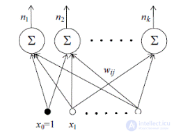
Figure 2.4 - Perseptron Rosenblatt.
Input neurons are usually designed to distribute the input signals between other neurons of the network, so they require that the signal coming from the element be the same as the incoming one. Unlike other neurons of the network, the inputs have only one input. In other words, each input element can receive a signal from one corresponding sensor. Since the input elements are intended solely to distribute signals received from the external environment, many researchers do not consider input elements to be part of the neural network at all.
Perceptron is able to solve linear problems. The number of network inputs determines the dimension of the space from which the input data is selected: for two features, the space is two-dimensional, for three features - three-dimensional, and for d features - d-dimensional. If a straight or hyperplane in the input data space can divide all samples into their corresponding classes, then the problem is linear, otherwise non-linear. Figure 2.5 shows the sets of points on the plane, and in case a) the boundary is linear, in case b) non-linear.

a) b)
Figure 2.5 - The geometric representation of the linear (a) and
nonlinear (b) problems.
To solve nonlinear problems, multilayer perceptron (MLP) models have been proposed that can construct a broken line between recognizable images. In multilayer networks, each neuron can send an output signal only to the next layer and receive input signals only from the previous layer, as shown in Figure 2.6. The layers of neurons located between the input and output are called hidden, because they do not receive or transmit data directly from the external environment. This network allows you to highlight the global properties of the data due to the presence of additional synaptic connections and increasing the level of interaction of neurons.

Figure 2.6 - Layout of a multilayer perceptron.
Determining the number of hidden layers and the number of neurons in each layer for a specific task is an informal problem, which can be solved using the heuristic rule: the number of neurons in the next layer is two times less than in the previous one
Currently, in addition to the multilayer perceptron, there are many ways to define the structures of neural networks. All types of neural networks can be divided into direct distribution networks and feedback networks. As the name implies, in networks of the first type, signals from a neuron to a neuron propagate in a clearly defined direction - from the network inputs to its outputs. In networks of the second type, the output values of any neuron of the network can be transmitted to its inputs. This allows the neural network to model more complex processes, for example, temporary ones, but it makes the outputs of a similar network unstable, depending on the state of the network in the previous cycle. In Figure 2.7. The classification of the most common types of neural networks is presented.

Figure 2.7 - Classification of common types of ANN.

Comments
To leave a comment
Intelligent Information Systems
Terms: Intelligent Information Systems