Lecture
F. Rosenblatt suggested using a perceptron for classification tasks. Many applications can be interpreted as classification problems. For example, optical character recognition. Scanned characters are associated with their respective classes. There are many variants of the image of the letter "H" even for one specific font - the symbol may turn out to be blurry, for example - but all these images must belong to the "H" class.
When it is known which class each of the learning examples belongs to, you can use a learning strategy with a teacher. The task for the network is to teach it how to match the sample presented to the network with the control target sample representing the desired class. In other words, environmental knowledge is represented by a neural network in the form of input-output pairs. For example, the network can show the image of the letter "H" and train the network so that the corresponding "H" output element must be turned on, and the output elements corresponding to other letters are turned off. In this case, the input sample can be a set of values characterizing the image pixels in grayscale, and the target output sample can be a vector, the values of all coordinates of which must be equal to 0, except for the coordinates corresponding to the class "H", the value of which must be equal.
Figure 3.1 shows a block diagram illustrating this form of learning. Suppose that a learning vector from the environment is supplied to the teacher and the learning network. Based on the built-in knowledge, the teacher can form and transmit the desired response corresponding to this input vector to the learning neural network. Network parameters are adjusted for the training vector and error signal. The error signal is the difference between the desired signal and the current response of the neural network. After graduation, teachers can turn off and allow the neural network to work with the environment on their own.

Figure 3.1 - The concept of learning ANN with a teacher.
The perceptron learning algorithm includes the following steps:
· The system is presented with a reference image.
· If the recognition result coincides with the specified one, the weighting coefficients of the links do not change.
· If the INS does not correctly recognize the result, then the weighting factors are incremented in the direction of improving the quality of recognition.
In the untrained network, randomly selected low weight values are assigned to relations. The difference between the known value of the result and the response of the network corresponds to the magnitude of the error, which can be used to adjust the weights of the interneuron links. The adjustment consists in a small (usually less than 1%) increase in the synaptic weight of those connections that enhance the correct reactions, and a decrease in those that contribute to erroneous ones.
We introduce the following notation:
X is the input vector from the external environment;
Y is the actual response of the perceptron;
D - desired output - the desired perceptron response.
The error signal initiates the procedure of their change, which is aimed at bringing the actual response to the desired one. If the perceptron contains k neurons, then the vectors in the expression Y and D have dimension k, and each coordinate corresponds to one neuron. In the process of learning, the energy of the total error is minimized, i.e. the sum of errors for all samples presented by the network at the training stage:
 (3.1)
(3.1)
Where p is the sample number,
k is the dimension of the vectors Y and D.
The rms error energy is the error energy per one example:
 (3.2)
(3.2)
Where M is the number of teaching examples.
The time during which all examples from the training sample are run through the network is called an epoch .
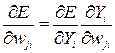
The minimization of a function is carried out according to the delta rule, or the Widrow-Hoff rule. Denote by w ji (n) the current value of the synaptic weight w ji of the neuron i corresponding to the input x j at the training step n . In accordance with the delta rule, the change in synaptic weight is given by the expression:
 (3.3)
(3.3)
Where η is a positive constant affecting the speed of learning.
This rule is easily derived in the case of the linear transfer function of neurons. The total error equation defines a multidimensional surface. In the process of learning, the network changes the weights so that a gradient descent along the surface of errors occurs. The surface gradient of weight error is expressed as follows:
 (3.4)
(3.4)
Because:
 ; (3.5)
 . (3.6)
Designating  , we obtain the expression for the error surface gradient:
 . (3.7)
The gradient indicates the direction in which the rate of rise of the error function is maximum. Multiplying the gradient by the speed of learning, and also considering that the movement along the surface of the error is towards the antigradient (after all we are looking for a minimum, isn’t it?), We get:
 (3.8)
(3.8)
Verbally delta rule can be defined as follows:
The correction applied to the neuron synaptic weight is proportional to the product of the error signal and the input signal that caused it:
 (3.9)
(3.9)
The step-by-step adjustment of the neuron's synaptic weights continues until the network reaches a steady state at which the weights are almost stabilized. At this point, the learning process stops.
Learning by example is characterized by three basic properties: capacity, sample complexity, and computational complexity. Capacity corresponds to the number of samples that can remember the network. The complexity of the samples determines the ability of the neural network to learn. In particular, when training ANNs, “overtraining” (“retraining”) conditions can occur in which the network functions well with examples of the training sample, but does not cope with new examples, losing the ability to learn.
The multilayer perceptron is able to solve arbitrary tasks. But for a long time its use was difficult due to the lack of an effective learning algorithm. With several layers of custom scales, it becomes unclear exactly what weights to adjust depending on the network error at the output. In 1986, Rumelhart, Hinton, and Williams proposed the so-called back-propagation algorithm.
The back propagation algorithm defines two streams in the network: the forward stream, from the input layer to the output layer, and the reverse flow - from the output layer to the input layer. A direct stream, also called a functional stream, pushes the input signals through the network, with the result that the output values of the network are obtained in the output layer. The reverse flow is similar to the forward flow, but it pushes the error values back through the network, as a result of which the values are determined, according to which the weights should be adjusted in the learning process. In the reverse flow, the values pass through the weighted links in the direction opposite to the direction of the forward flow. The presence of a double stream in the network is illustrated in Fig. 3.2.
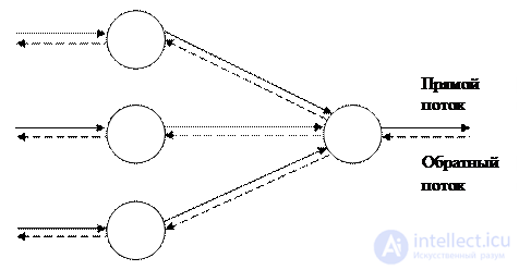
Figure 3.2 - Dual network stream.
The error signal of the output layer is calculated in the same way as in the case of a single-layer perceptron, since the reference values for the output layer are known and the error energy is calculated directly. If the neuron is located in a hidden network layer, the desired response for it is unknown. Consequently, the error signal of a hidden neuron must be recursively calculated based on the error signals of all neurons with which it is directly connected.
Let us denote the error of a neuron in some layer j as follows:
 ; (3.10)
where p j = Σw ji z i - the weighted sum of the inputs of the neuron;
z i - the inputs of the neuron and, accordingly, the outputs of the previous layer of neurons.
Applying the rule of differentiation of complex functions, we find the expression for the value of the neuron error in the output layer:
 (3.11)
For a neuron in the hidden layer, the expression is derived taking into account that the neuron sends a signal to the neurons in the next layer, for which the error is calculated from expression (3.11):
 (3.12)
Thus, the error at each layer is calculated recursively through the error values at the previous layers: error correction is propagated back through the neural network.
The energy function of the error E P is a rather complex gully surface with a large number of local minima (Fig. 3.3). If during a gradient descent to get to such a minimum, then, obviously, the network will not be tuned for optimal performance.
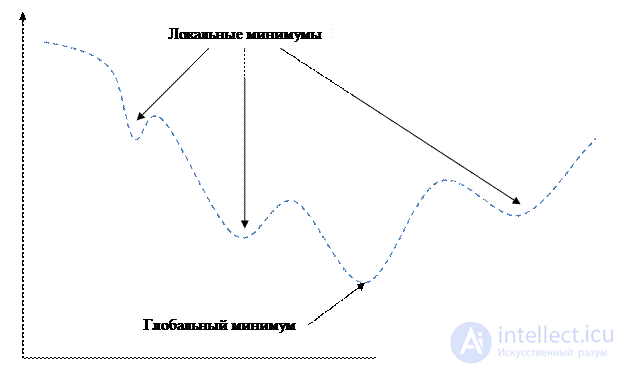
Figure 3.3 - Function with a ravine effect
There are several ways to solve problems associated with local minima.
1. The simplest method is to use the variable learning rate η. At the beginning of the algorithm, its value is a large value, close to 1. As η converges, it gradually decreases. This allows you to quickly reach a minimum, and then just get into it.
2. "Ravine" method. The trends in the surface are taken into account by adding the moment of inertia:
 (3.13)
Where μ is a positive number, called the moment constant.
Expression (3.13) is called the generalized delta rule. The idea is to jump through local minima at the surface of the error.
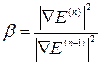
3. The conjugate gradient method. Fletcher and Reeves suggested choosing a direction conjugate to a gradient that more precisely indicates the minimum of the function:
 (3.14)
Where  - vector differential operator;
4. The most accurate solution is a solution that can be obtained from the so-called second-order methods. The general principle of operation is based on the use of a matrix of second derivatives - Hessian  .
.

Comments
To leave a comment
Intelligent Information Systems
Terms: Intelligent Information Systems