Models of neural networks .6. Hopfield network. Associative memory

Teaching without a teacher. Hebb's rule

Associative memory is a distributed memory that is trained on the basis of associations, like the brain of living beings. There are two types of associative memory: autoassociative and heteroassociative . When solving the problem of auto-associative memory, images (vectors) transferred to it are remembered in the neural network. Then, incomplete descriptions or noisy representations of the original images stored in memory are consistently submitted to this network, and the task of recognizing a particular image is posed. Hetero-associative memory differs from auto-associative memory in that a different set of output signals is assigned to the set of input images.

Let xk be the key image (vector) used to solve the problem of associative memory, and yk be the memorized image (vector). The relationship of the association of images realized by such a network can be described as follows: y k ↔ x to where q is the number of images stored in the network. The key image X * acts as a stimulus, which not only determines the location of the memorized image of k , but also contains the key for its extraction.

In the auto-associative memory, y k = xk. This means that the input and output spaces of the network must have the same dimension. In the heteroassociative memory, yk ≠ xk . This means that the dimension of the space of output vectors may differ from the dimension of the space of input vectors, but may also coincide with it.

For setting up neural networks intended for solving problems of auto-associative memory, training without a teacher is used, and in networks of heteroassociative memory - training with a teacher.

One of the first approaches used when teaching ANN without a teacher is D. Hebba's rule, which in the neurophysiological aspect is formulated as follows:

If the axon of cell A is located close enough to cell B and constantly or periodically participates in its excitation, then there is a process of metabolic changes in one or both neurons, expressed in the fact that the effectiveness of neuron A as one of the causative agents of neuron B increases.

Applied to artificial neural networks:

1. If two neurons on both sides of the synapse are activated synchronously (i.e., simultaneously), then the synaptic weight of this compound increases.

2. If two neurons on both sides of the synapse are activated asynchronously, then such a synapse is weakened or disconnected altogether.

The simplest form of training Hebb has the following form:

(6.1)

where y j is the element output from the previous one, and at the same time is the input for the neuron i;

w ji is the weight of the input of the neuron i, according to which the signal from the neuron j is received.

A significant disadvantage of this implementation: it is possible to increase the strength of communication, which leads to unstable network operation. More perfect implementations:

- covariance training: the deviations of the signals from the average values ​​over a short period of time are used;

- differential learning: the deviations of the signal values ​​from the values ​​at the previous iteration are used;

- learning with forgetting, γ - forgetting speed parameter, not more than 0.1.

Hopfield network

Consider a single neuron with feedback. At the first stage of the work, the input values ​​are fed to the input of the neuron and the output of the neuron is calculated. Then, the resulting output value is fed to the input of the neuron along with other values, and a new output value is calculated. This process is repeated until the output value of the neuron changes little from iteration to iteration.

If you go back to neural networks, you can enter the following classification. Recurrent neural networks, for which it is possible to obtain outputs stabilizing to a certain value, are called stable, and if the outputs of the network are unstable, then they are unstable. In general, most recurrent neural networks are unstable. Unstable networks are not very suitable for practical use.

In 1982, D. Hopfield proposed a stable recurrent INS architecture, shown in Figure 6.2. The Hopfield network has the following characteristics:

o The network is bipolar, that is, it operates only with values ​​taking the values ​​{–1, 1} or {0, 1}.

o The network has one layer of custom neurons. Moreover, the weights matrix is ​​symmetric.

o Each neuron is associated with all other elements, but is not associated with itself, therefore there are zero elements on the main diagonal of the weights matrix.

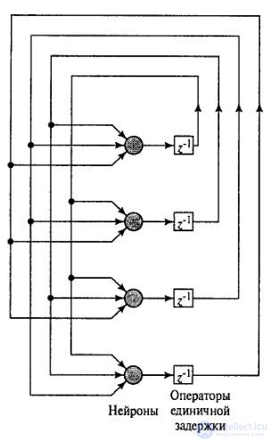
Figure 6.2 - Hopfield Network.

Initially, all memorized images x j , j = 1, ..., M, are encoded by bipolar vectors of length N. These vectors are called cells of the fundamental memory. Then the weights of the Hopfield network are configured directly from the input based on Hebb's rule:

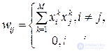, (6.2)

Where - i-th and j-th components of the k-th memorized sample.

At this point, the image memorization phase of the Hopfield network ends.

The matrix W has the following properties:

- is symmetric about the main diagonal: w ij = w ji ;

- the elements of the main diagonal are zero: w ii = 0;

At the beginning of the extraction phase, the initial states of the neurons are established in accordance with the input vector - the probe. A probe may represent a partially distorted image from network memory. Then the network works until it stabilizes in one of the stored states, the attractors. The output values ​​here are the restored association. It should be noted that if the input vector is strongly distorted, the result may be incorrect.

In the extraction phase, the following actions occur. The item to be updated is randomly selected. The selected element receives the weighted signals of all the remaining elements and changes its state according to the following rule:

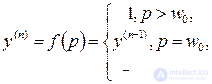(6.3)

where n is the iteration number.

Another element is selected, and the process is repeated. The network reaches the limit when none of its elements, being selected to update, changes its state. Items are updated randomly, but on average, each item must be updated to the same extent. For example, in the case of a network of 10 items after 100 updates, each item should be updated approximately 10 times.

Of particular interest is the network capacity. Theoretically, you can memorize 2N images, but in reality it turns out a lot less. It was experimentally obtained, and then it was theoretically shown that, on average, for weakly correlating images, a network of N neurons is able to remember ≈ 0.15N images.