Lecture
The basic idea of networks based on radial basis functions (RBF) is the nonlinear transformation of input data in a space of higher dimension. The theoretical basis of this approach is the Cover theorem on the separability of images:
Nonlinear transformation of a complex problem of pattern classification into a space of higher dimension increases the probability of linear separation of patterns.
RBF networks originate from the theory of exact approximation of functions proposed by Powell in 1987. Let a set of N input vectors x n be given with corresponding outputs y n . The task of exact approximation of functions is to find a function y such that y (x n ) = y n , n = 1, ..., N. For this, Powell suggested using a set of basis functions of the form  , then we obtain a generalized polynomial of the form:
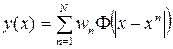 (5.1)
(5.1)
Here w n - freely adjustable parameters.
Usually, the exponential function is used as the base function. 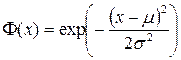 , also called the Gauss function, where μ and σ are the control parameters, called the center and width of the function window, respectively.
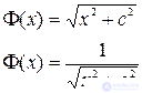
Also, as the basis functions, the multiquadratic and inverse multiquadratic functions are used, respectively:
The approximation of the unknown function y (x) using Gauss functions is shown in Fig. 5.1. In this figure, the red curve is represented by the sum of blue Gaussian, it is clear that for some point x the main contribution comes from only a few Gaussian, whose centers are close to this point. Therefore, such an approximation is called local.

Figure 5.1 - Local approximation of the function.
Approximation of the function by the formula (5.1) gives poor results for noisy data, therefore in 1988 D. Brumhead and D. Lowe proposed the RBF network model. The network with radial basis functions (RBF network) in its simplest form is a network with three layers: an input layer, one hidden layer and an output layer. The hidden layer performs a non-linear transformation of the input space into the hidden. In most cases, but not always, the number of neurons in the hidden layer is greater than the dimension of the input space. The output layer performs a linear transformation of the output of the hidden layer, i.e. its neurons always use a linear activation function.
A radial basis function Φ (x) is associated with each hidden element. Each of these functions takes a combined input and generates an activity value supplied to the output.
The links of the hidden layer element define the center of the radial function for this hidden element. In the RBF network, the activation of neurons is given by the distance (Euclidean norm) between the weight vector and the sample specified in the learning process:
 (5.2)
(5.2)
The weight vector w j serves as the center of the radial basis function corresponding to the neuron number j. Therefore, we denote it as μ j .
Rules of the job and training RBF network
1. The number M of basic functions is chosen much less than the number of training data: M << N. Here, the exponential function is also taken as the base function:
 (5.3)
(5.3)
2. The centers of the basis functions μ j do not rely on the points of the input data, i.e. do not match any of the input vectors. The definition of function centers becomes part of the learning process.
3. For each of the M basis functions, its own window width σ j is defined, which is also determined during the learning process of the RBF network. As a rule, the value of σ j is made slightly larger than the distance between the centers of the corresponding basis functions μ j .
4. In the sum (5.1), the constant w k0 is added - the neuron threshold and the formal hidden neuron Φ 0 (x) = 0 . As a result, the RBF network will be described by the formula:
 (5.4)
(5.4)
RBF network training is fast and carries elements of both learning with a teacher and without a teacher.
We have a training set: the set of inputs {x n } and the corresponding outputs {d n }. At the first stage, the parameters of the basis functions are determined: μ j , σ j . Moreover, only input vectors {x n } are used, i.e. training takes place according to the “without teacher” scheme.
To determine σ j , the “nearest neighbor” algorithm is used, which consists in searching for a partition of the set {x n } into M non-adjacent subsets of S j . Thus, it is necessary to minimize the function:
 where
where  - function centers.
At the second stage, the basic functions are fixed, i.e. the parameters μ j , σ j are constant. At this stage, the RBF network is equivalent to a single-layer neural network. Then learning takes place according to the rule of learning with the teacher. Error energy expression:

Since E is a quadratic function of the weights of w, the minimum of E can be found by solving a system of linear equations:

The solution of such a system is fast, and this is one of the advantages of the RBF network over a multilayer perceptron.
Among the shortcomings of the RBF network as compared to the MLP, the following is usually noted: more training examples are required, and the range of tasks to be solved is limited by approximation and classification.
The construction of neural networks according to the cascade correlation algorithm begins with a perceptron. The algorithm can be divided into two parts: the training of perceptron neurons and the creation of new neurons.
At the initial stage, when the perceptron is trained, after a significant decrease in the error does not occur for a given number of epochs, a decision is made to create a new neuron.
In the second part of the algorithm, a new candidate neuron is added to the existing network, and its inputs are connected to all the inputs of the network and the outputs of previously added candidate neurons. The input weights of the candidate are configured in a special way so as to minimize the error at the output of the resulting network. Figure 5.2 shows a network with two added neurons.
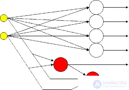
Figure 5.2 - Cascade Correlation Network.
The method was given this name because the sum of the correlations of its output with the values of existing neurons is used to tune the weights of the neuron candidate:

where y p is the output of the candidate neuron;
 - error of the output neuron j for sample p;
 - averaged over the sample values of the corresponding values.
The purpose of training is the maximum of the functional S. For this, its partial derivatives are calculated by the weights of the candidate neuron:

where λj is the sign of the correlation (+ or -) between y p and ;
I - the output value of the neuron added in the previous step.

Comments
To leave a comment
Intelligent Information Systems
Terms: Intelligent Information Systems