Hamming net

When there is no need for the network to explicitly produce a sample, that is, it is enough, say, to get a sample number, the associative memory is successfully implemented by the Hamming network. This network is characterized, compared to the Hopfield network, by lower memory costs and computational volume, which is evident from its structure.

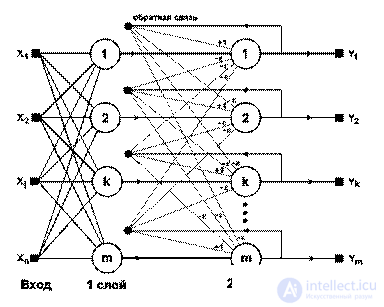
Figure 7.1 - Hamming Network.

The network consists of two layers. The first and second layers each have m neurons, where m is the number of samples. The neurons of the first layer have n synapses each connected to the network inputs (forming a dummy zero layer). The neurons of the second layer are interconnected by inhibitory (negative feedback) synaptic connections. A single synapse with positive feedback for each neuron is connected to its own axon.

The idea of ​​the network is to find the Hamming distance from the test image to all samples. The Hamming distance is the number of distinct bits in two binary vectors. The network must select a sample with a minimum Hamming distance to an unknown input signal, with the result that only one network output will be activated corresponding to this sample.

At the initialization stage, the weights of the first layer and the threshold of the activation function are assigned the following values:

, i = 1 ... n, k = 1 ... m;

w _{0 k} = n / 2, k = 1 ... m.

where x _i ^k is the i-th element of the k-th sample.

The weighting factors of the decelerating synapses w _ij , i ≠ j, in the second layer are assumed to be equal to some value 0 ii = 1.

The algorithm of the functioning of the Hamming network is as follows:

1. An unknown vector X = {xi: i = 1 ... n} is fed to the network inputs, from which the states of the first layer neurons are calculated:

, j = 1 ... m.

After that, the obtained values ​​initialize the values ​​of the axons of the second layer: y2 _j = y1 _j , j = 1 ... m.

2. Calculate the new states of the neurons of the second layer:

3. Check whether the outputs of the neurons of the second layer have changed during the last iteration. If yes, go to step 2. Otherwise, end.

From the evaluation of the algorithm, it is clear that the role of the first layer is very conditional: using the values ​​of its weights once in step 1, the network no longer refers to it, so the first layer can be excluded from the network altogether and replaced with a matrix of weights.

Bidirectional associative memory

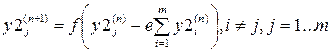
The associative memory implemented by the Hopfield network is auto-associative: the image stored in the network can be restored by a distorted input (the same vector), but not associated with an arbitrary other way. In 1980 - 83 years. S. Grossberg published a series of works on the so-called bidirectional associative memory.

Figure 7.2 - Network bidirectional associative memory.

Bidirectional associative memory (DCA) is actually a combination of two layers of the Hopfield network. In this case, a heterrassociation of two vectors A and B occurs. Associated images A and B are encoded by binary vectors of length n1 and n2, respectively. Then the network weight of the WCT is given by

To restore the association, the input vector A is fed to the inputs of layer 1 and processed by the weights matrix W; as a result, vector B must be formed at the layer output:

B = f (AW)

where f () is the transfer function (6.3).

The input vector of layer 2 B is processed by the matrix of weights W ^T , as a result, the output of layer 2 forms vector A, which is then transmitted to the inputs of layer 1:

A = f (BW ^T ),

where W ^T is the transposition of the matrix W.

The cycle is repeated until the DCA network stabilizes, that is, neither vector A nor vector B changes from iteration to iteration. As a result, the value of vector B will be the desired association to vector A.

The memory capacity of the DAD, represented by a network with N neurons in a smaller layer, can be estimated by the following value:

L 2 N).

DAP capacity is low, for N = 1024 neurons, the network will be able to memorize 50 patterns.

Boltzmann machine. Stochastic neuron model

The Boltzmann Learning Rule, named after Ludwig Boltzmann, is a stochastic learning algorithm based on the ideas of stochastic mechanics. The neural network created on the basis of Boltzmann’s training is called the Boltzmann machine. In its basic form, the Boltzmann machine is a Hopfield network using a stochastic model of neurons.

In a Boltzmann machine, neurons can be in the on (corresponding to +1) or off (-1) state. A machine is characterized by a function of energy, the value of which is determined by the specific states of the individual neurons that make up this machine:

The work of the machine is to perform the following actions:

- random selection of some neuron j at a certain step of the learning process;

- transfer of this neuron from state xj to state - xj with probability:

Where ΔE _J is the change in the energy of the machine caused by the change in the state of the neuron j: ;

T - pseudo-temperature, which does not describe the physical temperature of a natural or artificial network, but is a parameter of synaptic noise . The smaller the synaptic noise, the more the stochastic neuron approaches the deterministic one. With repeated application of this rule, the machine reaches thermal equilibrium.

The neurons of the Boltzmann machine can be divided into two functional groups. Visible neurons implement the interface between the network and the environment of its operation, while the hidden ones operate independently of the external environment. Consider two modes of operation of such a network.

• The constrained state (fixation phase), in which all visible neurons are in states predetermined by the external environment (ie, the input and the target associated output are set).

• Free state (free execution phase), in which only the input vector is fixed, and the network is working until the output values ​​stabilize.

During both phases, statistics are collected, which are used to change the weights of the links according to the Boltzmann rule:

,

Where - correlation between the states of neurons j and i in the constrained state;

- - in a free state.