5. Fourier transform for a one-dimensional signal. Fourier transform properties.

Fourier transform allows you to represent almost any function or data set as a combination of trigonometric functions such as sine and cosine, which allows you to identify periodic components in the data and evaluate their contribution to the structure of the original data or the form of the function. Traditionally, there are three main forms of the Fourier transform: the integral Fourier transform, the Fourier series and the discrete Fourier transform.

The Fourier integral transform converts a real function into a pair of real functions or one complex function into another.

The real function f (x) can be decomposed into an orthogonal system of trigonometric functions, that is, can be represented as

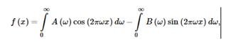
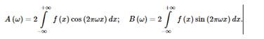
where A (ω) and B (ω) are called integral cosine and sine transforms:

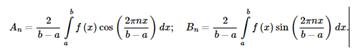
The Fourier series represents a periodic function f (x), given on the interval [a, b], in the form of an infinite series in sines and cosines. That is, an infinite sequence of Fourier coefficients is assigned to the periodic function f (x)

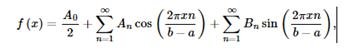
Where

The discrete Fourier transform translates a finite sequence of real numbers into a finite sequence of Fourier coefficients.

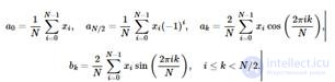
Let {xi}, i = 0, ..., N − 1 be a sequence of real numbers — for example, samples of brightness of pixels along an image line. This sequence can be represented as a combination of finite sums of the form

Where

The main difference between the three forms of the Fourier transform is that if the integral Fourier transform is defined over the entire domain of the function f (x), then the series and the discrete Fourier transform are defined only on a discrete set of points that is infinite for a Fourier series and finite for a discrete transform.

As can be seen from the definitions of the Fourier transform, the discrete Fourier transform is of greatest interest for digital signal processing systems. Data received from digital media or information sources are ordered sets of numbers written in the form of vectors or matrices.

It is usually assumed that the input data for the discrete transform is a uniform sample with a step Δ, while the value T = NΔ is called the record length, or the main period. The fundamental frequency is 1 / T. Thus, in a discrete Fourier transform, the input data is decomposed into frequencies that are an integer multiple of the fundamental frequency. The maximum frequency determined by the dimension of the input data is 1 / 2Δ and is called the Nyquist frequency . Accounting for the Nyquist frequency is important when using the discrete transform. If the input data has periodic components with frequencies higher than the Nyquist frequency, then when calculating the discrete Fourier transform, the high-frequency data will be replaced by a lower frequency, which can lead to errors when interpreting the results of the discrete transform.

An important tool for analyzing data is also the energy spectrum . The signal strength at frequency ω is determined as follows:

This value is often called the energy of the signal at the frequency ω. According to the Parseval theorem, the total energy of the input signal is equal to the sum of the energies at all frequencies.

The plot of power versus frequency is called the energy spectrum or power spectrum. The energy spectrum allows us to detect the hidden periodicities of the input data and evaluate the contribution of certain frequency components to the structure of the original data.

Fourier Transform Properties

The properties of the Fourier transforms determine the mutual correspondence of the transformation of signals and their spectra.

1. Linearity. The Fourier transform refers to the number of linear integral operations, i.e. the spectrum of the sum of the signals is equal to the sum of the spectra of these signals.

a _n s _n (t) <=> a _n S _n (w). (4.3.1)

An example of the summation of signals and its display in the spectral region in Fig. 4.3.1.

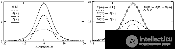
Fig. 4.3.1. Signals and their spectra. s0 (k) = s1 (k) + s2 (k) <=> S1 (w) + S2 (w) = S0 (w).

.

S (t) signal	Spectrum S (w)
Even	Real, even
Odd	Imaginary odd
Arbitrary	The real part is even. The imaginary part is odd

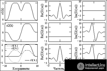
2. The symmetry properties of the transformation are determined by the cosine (even, real) and sine (odd, imaginary) parts of the decomposition and the similarity of the direct and inverse transformations.

In fig. 4.3.2. Examples illustrating the parity properties of the transformation are given. The signal s1 (k) is even, s1 (k) = s1 (-k), and has only real even spectrum (the imaginary part of the spectral function is represented by zero values). The signal s2 (k) = -s2 (-k) is odd and has an imaginary odd spectrum, and its real part is represented by zero values. The signal s3 (k) is formed by the sum of the signals s1 (k) and s2 (k). Accordingly, the spectral function of the signal is represented by both the real even part (belonging to s1 (k)) and the imaginary odd part (belonging to s2 (k)). When the inverse Fourier transform separates the real and imaginary parts of the spectrum S3 (w), as well as any other complex spectra, the even and odd parts of the original signal will be separately reconstructed.

An arbitrary source signal can be set in a one-way version (0-T), but the even and odd parts of this signal occupy the interval from –T to T, while on the left half of the numerical axis (from –T to 0) these two signals compensate each other giving zero values.

3. A change in the function's argument (compression or expansion of the signal) leads to the inverse change in the argument of its Fourier transform and inversely proportional to the change in its modulus. So, if s (t) Û S (w), then when changing the duration of the signal while maintaining its shape (stretching the signal along the time axis), i.e. for the signal with the new argument s (x) = s (at) with x = at, we get:

s (at) <=> s (at) exp (-jwt) dt = (1 / a) s (x) exp (-jxw / a) dx

s (at) <=> (1 / a) S (w / a). (4.3.2 ')

The expression (4.3.2 ') is valid for a> 0. When a <0, the mirror rotates the signal about the vertical axis, and changing the variable t = x / a causes a rearrangement of the integration limits and, accordingly, a change in the sign of the spectrum:

s (at) <=> - (1 / a) S (w / a). (4.3.2 '')

Generalized formula for changing the argument:

s (at) <=> (1 / | a |) S (w / a), a ≠ 0 (4.3.2)

If the argument of a function and its spectrum is to understand certain physical units, for example, time is frequency, then it follows: the shorter the signal is in duration, the wider is its spectrum in frequency, and vice versa. This can be clearly seen in fig. 4.3.1. for signals s1 (k) and s2 (k) and their spectra S1 (w) and S2 (w).

From the change in the argument of the functions, one should distinguish the change in the scale of the representation of functions. Changing the scale of the arguments changes the digitization of the numerical axes for displaying the signals and their spectra, but does not change the signals and spectra themselves. So, with the scale of the time axis t = 1 second, the scale of the frequency axis is f = 1 / t = 1 Hertz, and with t = 1 μsec f = 1 / t = 1 MHz (t = at, f = 1 / at, a = 10 ^-6 ). '

4. The delay theorem. The delay (shift, offset) of the signal in the function argument by the interval t _o leads to a change in the phase-frequency function of the spectrum (phase angle of all harmonics) by -wt _o . Applying the change of the variable tt _o = x, we get:

s (tt _o ) <=> s (tt _o ) exp (-jwt) dt =

= s (x) exp (-jwx) exp (-jwt _o ) dx = S (w) exp (-jwt _o ). (4.3.3)

It is obvious that the amplitudes of the signal harmonics during its shift should not change. Taking into account the fact that | exp (-jwt _o ) | = 1, this also follows from (4.3.3):

| S (w) exp (-jwt _o ) | = | S (w) |.

The phase spectrum is shifted by -wt _o with a linear dependence on frequency:

S (w) exp (-jwt _o ) = R (w) exp [j (j (w)] exp (-jwt _o ) = R (w) exp [j (j (w) -wt _o )]. ( 4.3.4)

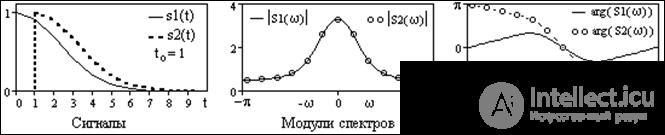
Fig. 4.3.3. The change in the spectrum of the signal during its shift.

An example of two identical signals shifted relative to each other by t _o = 1 and the spectra corresponding to these signals is shown in Fig. 4.3.3.

Similarly, it is easy to show that shifting the spectrum in the frequency domain by w ₀ causes the signal to multiply by exp (jw ₀ t):

S (w - w ₀ ) <=> s (t) exp (jw ₀ t),

which is equivalent to modulating the signal with the complex exponent function in the time domain.

5. Derivative Conversion (signal differentiation) :

s (t) = d [y (t)] / dt = d [Y (w) exp (jwt) dw] / dt = Y (w) [d (exp (jwt)) / dt] dw =

= jw Y (w) exp (jwt) dw <=> jw Y (w). (4.3.5)

The signal differentiation is displayed in the spectral region by simply multiplying the signal spectrum by the signal differentiation operator in the frequency domain jw, which is equivalent to differentiating each harmonic of the spectrum. Multiplication by jw enriches the spectrum of the derived signal with high-frequency components (compared to the original signal) and destroys components with zero frequency.

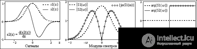
Fig. 4.3.4. Spectra of the signal and its derivative.

An example of a signal, its derivative and the spectra corresponding to them is shown in Fig. 4.3.4. By changing the spectrum argument (for an even source signal, it was zero), it can be seen that for all harmonics of the spectrum there is a phase shift of p / 2 (90 ⁰ ) for positive frequencies, and -p / 2 (-90 ⁰ ) for negative frequencies .

In general, for multiple derivatives:

d ⁿ [y (t)] / dt ⁿ = (jw) ⁿ Y (w). (4.3.6)

When differentiating the spectrum of a function, we respectively obtain:

d ⁿ [S (w)] / dw ⁿ = (-jt)  ⁿ s (t).

6. The transformation of the integral of the signal in the frequency domain with a known signal spectrum can be obtained from the following simple considerations. If takes place

s (t) = d [y (t)] / dt Û jw Y (w) = S (w),

then the inverse operation must be performed: y (t) = s (t) dt <=> Y (w) = S (w) / jw. This implies:

s (t) dt <=> (1 / jw) S (w). (4.3.7)

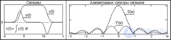
Fig. 4.3.5. Signals and amplitude spectra of signals.

The operator of integration in the frequency domain (1 / jw) at w> 1 weakens high frequencies in the amplitude spectrum and at w <1 strengthens low frequencies. The phase spectrum of the signal is shifted by -90 ⁰ for positive frequencies and by 90 ⁰ for negative. An example of the modulus of the signal spectrum and its integral function is shown in Fig. 4.3.5.

The formula (4.3.7) is valid for signals with a zero constant component. When integrating signals with a certain value of the constant component C = const, the additional term of the Fourier transform of the constant component C appears in the right-hand side of expression (4.3.7), which is a delta function at zero frequency with a weighting factor equal to the value of C:

(1 / jw) S (w) + C · d (0).

7. Conversion of convolution of signals y (t) = s (t) _* h (t):

Y (w) = y (t) exp (-jwt) dt = s (t) h (tt) exp (-jwt) dtdt.

Y (w) = s (t) dth (tt) exp (-jwt) dt.

By the delay theorem (4.3.3):

h (tt) exp (-jwt) dt = H (w) exp (-jwt).

From here: Y (w) = H (w) s (t) exp (-jwt) dt = H (w) · S (w).

s (t) _* h (t) <=> S (w) H (w). (4.3.8)

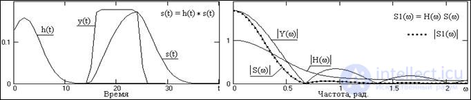
Fig. 4.3.6. Signals and amplitude spectra of signals.

An example of performing convolution in the frequency domain is shown in Fig. 4.3.6. Note that the frequency representation H (w) of the impulse response h (t) of the linear system (or the corresponding linear operation) has the meaning of the frequency transfer function of the system and allows determining the signal at the system output (in the frequency form of the representation) when specifying an arbitrary signal (in the frequency form ) at her entrance. Essentially, the function H (w) is the frequency distribution of the transmittance of the frequency components of the signal from the input to the output of the system.

Thus, the convolution of functions in the coordinate form is displayed in the frequency representation by the product of the Fourier transforms of these functions.

This provision is fundamental in data processing practice.

Any linear data processing system (information signals) implements a certain signal transformation operation, i.e. performs a convolution of the input signal s (t) with the operator of the system h (t). With the use of convolution transformation, this operation can be performed with both the dynamic and frequency forms of the representation of signals. At the same time, the processing of data presented in digital form is performed, as a rule, in the frequency domain, since may be several orders of magnitude higher in performance than in the time domain. It is a sequence of the following operations.

1. Translation of the signal into the frequency domain: s (t) Û S (w).

2. Multiplication of the signal spectrum by the transfer function of the system: Y (w) = H (w) · S (w).

The transfer function of the system is determined by a similar transformation h (t) Û H (w) or is specified directly in the frequency representation, which allows you to set the transfer functions of arbitrarily complex shapes, including those with discontinuities and jumps, for which h (t ) with infinite impulse response.

3. Translation of the spectrum of the processed signal into the time domain: Y (w) Û y (t).

8. Transformation of the product of signals y (t) = s (t) · h (t):

Y (w) = s (t) h (t) exp (-jwt) dt = s (t) [(1 / 2p) H (w ') exp (jw't) dw'] dt =

= (1 / 2p) s (t) H (w ') exp (-j (w-w') t) dw'dt =

(1 / 2p) H (w ') dw's (t) exp (-j (w-w ') t) dt =

= (1 / 2p) H (w ') S (w-w') dw '= (1 / 2n) H (w) _* S (w). (4.3.9)

Thus, the product of functions in the coordinate form is displayed in the frequency representation by convolving the Fourier transforms of these functions, with the normalization factor (1 / 2p), taking into account the asymmetry of the direct and inverse Fourier transforms of the functions s (t) and h (t) when using angular frequencies .

9. Derivative of convolution of two functions s' (t) = d [x (t) _* y (t)] / dt. Using expressions (4.3.6) and (4.3.8), we get:

s' (t) = jw [X (w) Y (w)] = (jw X (w)) Y (w) = X (w) (jw Y (w).

s' (t) = x '(t) _* y (t) = x (t) _* y' (t).

This expression allows the computation of the derived signal with simultaneous smoothing by a weighting function that is derived from the smoothing function (for example, Gaussian).

10. Power spectra. The time function of the signal power in general form is determined by the expression:

w (t) = s (t) s ^* (t) = | s (t) | ²

The spectral power density, respectively, is equal to the Fourier transform of the product s (t) · s ^* (t), which will be displayed in the spectral representation by convolving the Fourier transforms of these functions:

W (f) = S (f) _* S ^* (f) = S (f) S ^* (fv) dv. (4.3.10)

But for all current values ​​of frequency f, the integral in the right side of this expression is equal to the product S (f) · S ^* (f), since for all values ​​of the shift v ≠ 0, due to the orthogonality of the harmonics S (f) and S ^* (fv), the values their works are zero. From here:

W (f) = S (f) _* S ^* (f) = | S (f) | ² (4.3.11)

The power spectrum is a real non-negative even function, which is often called the energy spectrum. The power spectrum, like the square of the modulus of the signal spectrum, does not contain phase information about the frequency components, and, therefore, the restoration of the signal from the power spectrum is impossible. This also means that signals with different phase characteristics can have the same power spectra. In particular, the shift of the signal does not affect its power spectrum.

For the power functions of the interaction of signals in the frequency domain, respectively, we have the frequency power spectra of the interaction of signals:

W _xy (f) = X (f) Y * (f),

W _yx (f) = Y (f) X * (f),

W _xy (f) = W * _yx (f).

The power functions of the interaction of signals are complex, even if both functions x (t) and y (t) are real, while Re [W _xy (f)] is an even function, and Im [W _xy (f)] is odd. Hence, the total energy of interaction of signals when integrating the functions of the interaction power is determined only by the real part of the spectrum:

E _xy = (1 / 2p) W _xy (w) dw = (1 / n) Re [W _xy ] dw,

and is always a real number.

11. Equality Parseval. The total energy spectrum of the signal:

E _s = W (f) df = | S (f) | ² df. (4.3.12)

Since the coordinate and frequency representation is essentially only different mathematical mappings of the same signal, then the signal energy must be equal in two representations, from which Parseval equality follows:

| s (t) | ² dt = | S (f) | ² df,

those. the signal energy is equal to the integral of the modulus of its frequency spectrum — the sum of the energies of all the frequency components of the signal. Similarly for the energy of the interaction of signals:

x (t) y * (t) dt = X (f) Y * (f) df.

Из равенства Парсеваля следует инвариантность скалярного произведения сигналов и нормы относительно преобразования Фурье:

áx(t),y(t)ñ = áX(f),Y(f)ñ, ||x(t)|| ² = ||X(f)|| ²

Не следует забывать, что при представлении спектров в круговых частотах (по w) в правой части приведенных равенств должен стоять множитель 1/2п.