Lecture
A general representation of the transport problem (or the Hitchcock problem, or T-problem) is shown in the figure.
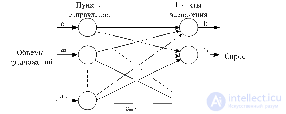
The transport task is shown as a network with m points of departure and n destinations, which are shown as network nodes.
The arcs connecting the network nodes correspond to the routes connecting the points of departure and destination. Two types of data are connected with arc (i, j) connecting point of departure i with destination j: the cost c ij of transportation of a unit of cargo from point i to point j and the amount of cargo carried x ij . The cargo volume at the point of departure i is equal to a i , and the cargo at destination point j is b j . The task is to determine the known values of x ij , minimizing the total transportation costs and satisfying the constraints on supply and demand.
So:  , (one)
under restrictions
 (2) (full withdrawal condition)
 (3) (condition for full satisfaction of demand)
Thus, the T-problem is an LP problem.
It is usually assumed that the total stock of cargo at the points of departure is equal to its total demand at the points of consumption. In this case, the T-problem is called balanced:  . (four)
The T-problem as an LP problem has mn variables and m + n constraints in the form of equalities. It turns out that not all m + n equations of the formulated problem are linearly independent. Indeed, summing all equations (2) and all equations (3), by virtue of condition (4), we get the same thing. Consequently, conditions (2) and (3) are interconnected by one linear dependence and the initial plan of the problem must contain m + n-1 non-zero components.
An example . The car company has three factories: in Los Angeles, Detroit and New Orleans and two warehouses in Denver and Miami. Production volumes for the quarter are respectively: 100, 1500 and 1200 cars. The weekly need for warehouses is 2300 and 1400 cars. Distances are shown in the table:
|
|
Denver |
Miami |
|
Los Angeles |
1000 |
2690 |
|
Detroit |
1250 |
1350 |
|
New Orleans |
1275 |
850 |
The transport company estimates its services at 8 cents for transporting one car for one mile. The cost of transportation is as follows (rounded to the dollar):
|
i |
Denver (1) |
Miami (2) j |
|
Los Angeles (1) |
80 |
215 |
|
Detroit (2) |
100 |
108 |
|
New Orleans (3) |
102 |
68 |
The task of the LP is formed as follows:
z = 80x 11 + 215x 12 + 100x 21 + 108x 22 + 102x 31 + 68x 32
under restrictions:
x 11 + x 12 = 1000 (L-A)
x 21 + x 22 = 1500 (Det)
x 31 + x 32 = 1200 (N.O.)
x 11 + x 21 + x 31 = 2300 (Den)
x 12 + x 22 + x 32 = 1400 (M)
x ij ≥0, i = 1,2,3; j = 1,2.
The task is balanced. T-task is recorded in the form of a so-called transport table.
|
|
Denver |
Miami |
Volume of production |
|
Los Angeles |
80 x 11 |
215 x 12 |
1000 |
|
Detroit |
100 x 21 |
108 x 22 |
1500 |
|
New Orleans |
102 x 31 |
68 x 32 |
1200 |
|
DEMAND |
2300 |
1400 |
|
The optimal solution is: 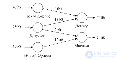
The minimum cost of transportation is 3/3 200 dollars.
When  The transport problem is called unbalanced. Any unbalanced task can be made balanced. For this, fictitious points of departure and destination are introduced.
Example. Let the plant in Detroit reduced production to 1,300 cars (instead of 1,500). The total quantity (3500) is less than the total quantity ordered (3700). Some orders of warehouses will not be fulfilled.
Since demand exceeds supply, in order to restore balance, we introduce a fictitious plant (point of departure) producing 3700-3500 = 200 machines. Since a fictitious plant does not exist, we assign a zero cost of transportation from it to the warehouses. In principle, this value can be any positive number. For example, to guarantee all orders for a warehouse in Miami, you can assign a very high shipping cost (fine) from a fictitious plant to Miami. This is a balanced model and its solution.
|
|
Denver |
Miami |
Volume of production |
|
Los Angeles |
80 1000 |
215
|
1000 |
|
Detroit |
100 1300 |
108
|
1300 |
|
New Orleans |
102
|
68 1200 |
1200 |
|
Dummy factory |
0 |
0 200 |
200 |
|
DEMAND |
2300 |
1400 |
|
The solution shows that a fictitious plant will deliver 200 cars to Miami (i.e., from an order of 1,400,200 vehicles will not be delivered)
Suppose a warehouse in Denver has ordered only 1,900 vehicles (supply exceeds demand). You must enter a fictitious destination, absorbing the difference. The cost of transportation may be zero, or a penalty (large), if you need to remove all products from this plant.
|
|
Denver |
Miami |
Dummy warehouse |
Volume of production |
|
Los Angeles |
80 1000 |
215
|
0 |
1000 |
|
Detroit |
100 900 |
108 200 |
0 400 |
1500 |
|
New Orleans |
102
|
68 1200 |
0 |
1200 |
|
DEMAND |
2300 |
1400 |
400 |
|
400 cars from Detroit are not in demand.
The solution of the transport problem.
In principle, as an LP problem, the T-problem can be solved by the simplex method. But it is solved by a special method, repeating the steps of the simplex method, but using transport tables.
Example. The transport company transports grain from 3 elevators to 4th mills. Task conditions are presented in the table. Shipping costs are in hundreds of dollars.
|
|
Mills |
|
|||
|
|
one |
2 |
3 |
four |
Sentence |
|
one |
ten x 11 |
2 x 1 2 |
20 x 1 3 |
eleven x 1 4 |
15 |
|
Elevators 2 |
12 x 2 1 |
7 x 22 |
9 x 23 |
20 x 24 |
25 |
|
3 |
four x 3 1 |
14 x 32 |
sixteen x 33 |
18 x 34 |
ten |
|
Demand |
five |
15 |
15 |
15 |
|
The sequence of solutions of the T-problem exactly repeats the scheme of the simplex algorithm.
Step 1. Determine the initial basic solution. Go to step 2.
Step 2. On the basis of the optimality condition of the simplex method among the nonbasic variables, we determine what is introduced into the basis . If all nonbasic variables satisfy the optimality condition, the calculations are complete. If not, go to step 3.
Step 3. Using the admissibility condition among the current basis variables, we determine the excluded one . We find a new basic solution. Go to step 2.
Definition of the initial decision.
As we said, there are m + n constraints in the form of equalities. Since the transport model is balanced, one of them should be redundant. Independent constraints m + n-1, the same number should be basic variables in the initial solution.
The special structure of the T-model for constructing the initial solution allows the following three methods to be applied.
1. Northwest corner method.
2. Least Cost Method
3. Vogel Method
Northwest corner method.
Execution starts from the top left cell (northwest corner) of the transport table, that is, with the variable x 11 .
Step 1. The variable x 11 is assigned the maximum value allowed by the constraints on supply and demand.
Step 2. A line (or column) is deleted with a fully realized proposal (with satisfied demand). This means that in the crossed out row (column) we will not assign values to the other variables (except the one defined in Step 1). If both supply and demand are satisfied at the same time, only the row or column is deleted.
Step 3. If only one row or only one column is not crossed out, the process is terminated. Otherwise, go to the cell on the right, if the column is crossed out, or to the cell down, if the row is crossed out. Then we return to the first stage. Last example:

Received initial baseline solution.
x 11 = 5; x 12 = 10; x 22 = 5; x 23 = 15; x 23 = 5; x 34 = 10.
Corresponding shipping cost:  Doll.
Doll.
The lowest cost method (minimum element method).
This method finds the best solution because it selects variables with which the minimum costs correspond. The entire table is searching for a cell with a minimum cost. The variable in this cell is assigned the maximum value of supply and demand. (If there are several such variables, the choice is arbitrary). The corresponding column (line) is deleted and the demand-supply is corrected accordingly.
If both demand and supply constraints are met at the same time, either the column or row is deleted. Not crossed out cells are viewed, a new cell is selected with a minimum cost. The process continues until only one row or column not crossed out remains.

1. Cell (1,2)  ($ 2). Cross out the second column. The demand supply of the first row of the second column is zero.
2. Further a cell (3,1).  Cross out the first column. The restriction of the third line on the proposal was 5
3. Cell (2,3)  15
15
4. Further  , x 34 = 5, x 24 = 10.
x 12 = 15; x 14 = 0; x 23 = 15; x 24 = 10; x 31 = 5; x 34 = 5.
 Doll.
Doll.
This is better than with the NW angle method.
Vogel method.
This is a variation of the minimum cost method, and in general gives the best solution.
Step 1. For each row (column), which corresponds to strictly positive supply (demand), the penalty is calculated by subtracting the lowest cost from the next highest value in the given row (column).
Step 2. Select the row or column with the highest penalty. If there are several, the choice is arbitrary. From the selected row or column, a variable is selected that corresponds to the minimum value, and it is assigned the highest value allowed by the constraints. Adjusted supply demand. The row or column corresponding to the constraint executed is deleted from the table. If both demand and supply constraints are fulfilled simultaneously, only one row or one column is deleted, and the remaining row (column) is assigned zero supply (demand).
Step 3.
a) If only one row or one column with zero demand and supply is not crossed out, the calculations end
b) If only one row (column) with a positive supply (demand) is not crossed out, basic variables are found in this row (column) using the least-cost method and the calculations are terminated.
c) If all unfused rows and columns correspond to zero volumes of supply and demand, the zero basis variables are found using the lowest cost method and the calculations are terminated.
d) In all other cases, go to step 1.
|
|
one |
2 |
3 |
four |
|
Fines for strings |
|
|
ten |
2 |
20 |
eleven |
15 |
10-2 = 8 |
|
|
12 |
7 |
9 |
20 |
25 |
9-7 = 2 |
|
|
four |
14 |
sixteen |
18 |
ten |
14-4 = 10 |
|
|
five |
15 |
15 |
15 |
|
|
|
Fines for columns |
10-4 = 6 |
7-2 = 5 |
16-9 = 7 |
18-11 = 7 |
|
|
The third line has the largest penalty (10). x 31 (min. cost) 5 Cross out the first column. Recalculated fines.
|
|
one |
2 |
3 |
four |
|
Fines for strings |
|
one |
ten |
2 |
20 |
eleven |
15 |
9 |
|
2 |
12 |
7 |
9 |
20 |
25 |
2 |
|
3 |
four |
14 |
sixteen |
18 |
five |
2 |
|
|
0 |
15 |
15 |
15 |
|
|
|
Fines for columns |
- |
five |
7 |
7 |
|
|
Now the first line (9) has the greatest penalty.
x 12 (min cost 2) 15. Constraints are performed for both the first row and the second column. Cross out the second column. The resource of the first row is zero. In the next step, the second line will have the largest penalty (20-9 = 11). x 23 (9) 10. Only the fourth column with a positive unsatisfied demand of 15 units is not crossed out. We apply the least cost method to it and we have x 14 = 0, x 34 = 5 and x 24 = 10.
Doll
The same value as in the previous method. But approximation is usually better.

Comments
To leave a comment
Mathematical methods of research operations. The theory of games and schedules.
Terms: Mathematical methods of research operations. The theory of games and schedules.