Lecture
Two rules for the choice of input and exclude variables in the simplex method are called the optimality condition and the admissibility condition.
Optimality condition. The variable introduced in the maximization (minimization) problem is a nonbasic variable having the largest negative (positive) coefficient in the Z-line. The optimal solution will be achieved when in the Z-line all coefficients with nonbasic variables are non-negative (non-positive).
The condition of admissibility. Both in the minimization problem and in the maximization problem, the base variable is chosen as excluded, for which the positive ratio of the value of the right side of the constraint to the positive coefficient of the leading column is minimal.
The sequence of actions in the simplex method:
Stage 0. The initial admissible basic solution is found.
Step 1. Based on the optimality condition, the input variable is determined. If there are no variables entered, the calculations end.
Step 2. Based on the validity condition, the excluded variable is selected.
Step 3. Calculate the new baseline solution. Go to item 1.
Artificial initial decision.
In the example of Reddy Mikks with an admissible initial basic solution, all subsequent basic solutions obtained by executing the simplex method will also be admissible. In problems of LP, where all restrictions are inequalities of the type "  »(With a nonnegative right-hand side) additional (residual) variables make it possible to form the initial admissible basic solution. And how to form it, if there are inequalities of the type "
  ". In this case, artificial variables are used. These variables in the first iteration play the role of additional residual variables, and then they are freed from them. Two methods have been developed for finding the initial solution using artificial variables: the M-method and the two-stage method.
M-method.
Let the LP problem be written in standard form. For any equality that does not contain an additional residual variable, we introduce an artificial variable R, which will then be included in the initial basic solution. But since this variable is artificial (it does not have a physical meaning in the problem), it is necessary to make it so that at subsequent iterations it vanishes. To do this, an expression is introduced into the expression of the objective function.
The variable R, with the help of a sufficiently large positive number M, is penalized by introducing the expression –MR 1 into the objective function in the case of maximization and + MR 1 in the case of minimization. Due to this penalty, it is reasonable to assume that the optimization process will lead to a zero value of R 1 .
Example.
Minimize z = 4x 1 + x 2
3x 1 + x 2 = 3
4x 1 + 3x 2 6
x 1 + 2x 2 four
x 1 x 2 0
We result in the standard form:
z = 4x 1 + x 2  min
min
3x 1 + x 2 = 3
4x 1 + 3x 2 -x 3 = 6
x 1 + 2x 2 + x 4 = 4
x 1 x 2 x 3 x 4 0
The first and second equations do not have additional residual variables that can be introduced into the basic solution. Therefore, we introduce artificial variables R 1 and R 2 into these equations, and we introduce the penalty MR 1 + MR 2 into the objective function.
z = 4x 1 + x 2 + MR 1 + MR 2
3x 1 + x 2 + R 1 = 3
4x 1 + 3x 2 -x 3 + R 2 = 6
x 1 + 2x 2 + x 4 = 4
x 1 , x 2 , x 3 , x 4 , R 1 , R 2 0
Basis | x 1 | x 2 | x 3 | R 1 | R 2 | x 4 | Decision |
z | -four | -one | 0 | -M | -M | 0 | 0 |
R 1 | 3 | one | 0 | one | 0 | 0 | 3 |
R 2 | four | 3 | -one | 0 | one | 0 | 6 |
x 4 | one | 2 | 0 | 0 | 0 | one | four |
Before applying the simplex method, you need to align the Z-string with the rest of the table. So Z, corresponding to the initial basis solution R 1 = 3, R 2 = 6 and x 4 = 4 should be 3M + 6M + 0 = 9M, not 0. The coefficients for R 1 and R 2 should be made zero. To do this, you need to multiply the lines R 1 and R 2 (all elements) by M, and then add these lines with a Z-line.
New Z-line = Old Z-line + M  R 1 - line + M R 2 is a string.
Basis | x 1 | x 2 | x 3 | R 1 | R 2 | x 4 | Decision |
z | -4 + 7M | -1 + 4M | -M | 0 | 0 | 0 | 9M |
R 1 | 3 | one | 0 | one | 0 | 0 | 3 |
R 2 | four | 3 | -one | 0 | one | 0 | 6 |
x 4 | one | 2 | 0 | 0 | 0 | one | four |
Now Z = 9M, which corresponds to the basic solution R 1 = 3, R 2 = 6 and x 4 = 4.
Since we solve the minimization problem, we choose the largest positive coefficient in the Z-line. It is -4 + 7M and corresponds to the variable x 1 , which will be entered. The condition of admissibility indicates that R 1 - excluded.
Basis | x 1 | x 2 | x 3 | R 1 | R 2 | x 4 | Decision |
z | 0 | (1 + 5M) / 3 | -M | (4-7M) / 3 | 0 | 0 | 4 + 2M |
x 1 | one | 1/3 | 0 | 1/3 | 0 | 0 | one |
R 2 | 0 | 5/3 | -one | -4/3 | one | 0 | 2 |
x 4 | 0 | 3/5 | 0 | -1/3 | 0 | one | 3 |
Already the first iteration has excluded from the basic solution R 1 - this is the result of a fine.
The next (input and exclude variable) will be x 2 and R 2 respectively. And the decision will be received.
When using the M-method, the following circumstances are important:
1. The use of a fine M may not lead to the elimination of an artificial variable. (For example, if the constraint system is incompatible).
2. Theoretically, the application of the M-method requires that M  . But from the point of view of computer calculations, M must be finite, but large enough. Large enough to fulfill the role of “fine”, but not too large so as not to reduce the accuracy of the calculations.
Two-step method.
It is devoid of the shortcomings that are inherent in the M-method due to rounding errors. The process of solving the problem is divided into two stages. At the first stage, a search is made for a feasible solution. If such a solution is found, then the initial problem is solved at the second stage.
Stage 1. The LP task is written in a standard form, and artificial variables are added to the constraints, as in the M-method. The LP problem is solved by minimizing the sum of artificial variables with initial constraints. If the minimum value of this new objective function is greater than zero, then the original problem has no feasible solution and the calculation process ends. If the new objective function is zero, go to the second stage.
Stage 2. The optimal basic solution obtained in the first stage is used as the initial admissible basic solution of the original problem.
Example (same task)
Stage 1. Minimize z = R 1 + R 2
3x 1 + x 2 + R 1 = 3
4x 1 + 3x 2 -x 3 + R 2 = 6
x 1 + 2x 2 + x 4 = 4
x 1 , x 2 , x 3 , x 4 , R 1 , R 2 0
Basis | x 1 | x 2 | x 3 | R 1 | R 2 | x 4 | Decision |
r | -four | -one | 0 | -one | -one | 0 | 0 |
R 1 | 3 | one | 0 | one | 0 | 0 | 3 |
R 2 | four | 3 | -one | 0 | one | 0 | 6 |
x 4 | one | 2 | 0 | 0 | 0 | one | four |
As in the M-method, a new r-string is first calculated:
New r-line = Old r-line + 1 R 1 is a string + 1 R 2 - string
The new r-string is used to solve the problem of the first stage.
Basis | x 1 | x 2 | x 3 | R 1 | R 2 | x 4 | Decision |
r | 0 | 0 | 0 | -one | -one | 0 | 0 |
x 1 | one | 0 | 1/5 | 3/5 | -1/5 | 0 | 3/5 |
x 2 | 0 | one | -3/5 | -4/5 | 3/5 | 0 | 6/5 |
x 4 | 0 | 0 | one | one | -one | one | one |
The minimum r = 0 is reached, which means that a valid basic solution x 1 = 3/5, x 2 = 6/5 and x 4 = 1 is obtained. Artificial variables have completed their mission and can be deleted.
Next step 2 is performed.
Duality in linear programming.
Each LP problem can be associated with a so-called dual problem.
The task of the LP in the standard form is:
Minimize or maximize

under restrictions:


The rules for the formation of a dual task:
1. To each of the m constraints of the direct problem there corresponds a variable of the dual problem.
2. Each of the n variables of the direct problem corresponds to a constraint.
dual task.
3. The coefficients for any variable in the constraints of the direct problem become the constraint coefficients of the dual problem corresponding to this variable, and the right side of the constraint being formed is equal to the coefficient for this variable in the objective function.
4. The coefficients of the objective function of the dual problem are equal to the right-hand sides of the constraints of the direct problem.
In the dual problem, the type of optimization of the objective function and the type of constraints change.
Example. Direct challenge
z = 5x 1 + 12x 2 + 4x 3 max
x 1 + 2x 2 + x 3 ten
2x 1 -x 2 + 3x 3 = 8
x 1 x 2 x 3 0
Direct challenge in standard form:
z = 5x 1 + 12x 2 + 4x 3 + 0x 4 max
x 1 + 2x 2 + x 3 + x 4 = 10
2x 1 -x 2 + 3x 3 + 0x 4 = 8
x 1 x 2 x 3 x 4 0
Dual Variables:
w = 10y 1 + 8y 2 min
y 1 + 2y 2 five
2y 1 -y 2 12
y 1 + 3y 2 four
y 1 + 0y 2 0
y 1 , y 2 - free  (y 1 0, y 2 - free variable)
Example. Direct challenge
z = 15x 1 + 12x 2 min
x 1 + 2x 2 3
2x 1 -4x 2 five
x 1 x 2 0
Direct challenge in standard form:
z = 15x 1 + 12x 2 + 0x 3 + 0x 4 min
x 1 + 2x 2 -x 3 + 0x 4 = 3
2x 1 -4x 2 + 0x 3 + x 4 = 5
x 1 x 2 x 3 x 4 0
Dual Variables: y 1 , y 2
Dual task:
w = 3y 1 + 5y 2 max
y 1 + 2y 2 15
2y 1 -4y 2 12
-y 1 0 (or y1 0)
y 2 0
y 1 , y 2 are free variables.
The meaning of the dual problem.
Let the task of optimal distribution of resources be given. Resources b 1 , b 2 ..b m can be used for the production of n types of products. The cost of the j-th type of product c j (j =) and the rate of consumption of the i-th resource (i =) per unit of product j - a ij are known . It is required to determine the volume of production of each type of product x j (j =), maximizing income
z = c 1 x 1 + c 2 x 2 + .. + c n x n
Resource consumption should not exceed their availability:
a 11 x 1 + a 12 x 2 + .. + a 1n x n b 1
------------------------------------------
 a i1 x 1 + a i2 x 2 + .. + a in x n b i
--------------------------------------- ---
a m 1 x 1 + a m 2 x 2 + .. + a mn x n b m
All variables are non-negative.
Assume that instead of production, you can sell raw materials to another buyer. The question is what minimum price should be set for a unit of each type of raw material (i =  ) provided that the income from the sale of all of its stocks should not be less than that which can be obtained from the production of products from this raw material. Consideration of the interests of the buyer is associated with minimizing the total cost of raw materials. The answer to this question gives a dual problem.
w = b 1 y 1 + b 2 y 2 + .. + b m y m min
a 11 y 1 + a 21 y 2 + .. + a m1 y m c 1
------------------------------------------
a 1j y 1 + a 2j y 2 + .. + a mj y m c j
------------------------------------------
a 1n y 1 + a 2n y 2 + .. + a mn y m c n
y i 0, (i = )
The variables y i of the dual task reflect the “value” of the i-th resource. In this regard, the variables of the dual task are called shadow prices or hidden incomes (sometimes simplex multipliers).
Dual to the dual task is direct. In the "direct - dual" system, both tasks are equivalent. Any of them can be considered as direct, then the second will be dual to it.
Basic duality theorems.
Theorem 1. If x 0 and y 0 are admissible solutions of the direct and dual problems, i.e. Ax 0 b and A T y 0 c then
c T x 0 b T y 0 ,
those. the values of the objective function of the direct problem never exceed the values of the objective function of the dual problem.
Theorem 2 (main duality theorem). If x 0 and y 0 are admissible solutions to the direct and dual problems and if c T x 0 = b T y 0 , then x 0 and y 0 are the optimal solutions of a pair of dual problems.
It is this theorem that binds the optimal solutions of the direct and dual problems. If in a direct problem with a small number of variables there is a large number of restrictions (m> n), it is more advantageous to solve the dual problem.
Theorem 3. If, in the optimal solution of the direct problem, the ith constraint is satisfied as a strict inequality, then the optimal value of the corresponding dual variable is zero.
The meaning is as follows: If some resource b i is abundant and the i-th inequality is fulfilled as a strict inequality, then it becomes insignificant and the optimal shadow price of such a resource is zero.
Theorem 4. If in the optimal solution of the dual problem the restriction j is fulfilled as a strict inequality, then the optimal value of the corresponding variable of the direct problem must be equal to zero.
We give an interpretation of Theorem 4. Since the quantities y i (i = ) - these are the prices of the corresponding resources,  - is the cost of the j-th process. The theorem then means the following: if the jth process turns out to be disadvantageous from the point of view of optimal prices for resources y opt , then in the optimal solution of the direct problem, the intensity of such a process must be zero. Theorem 4 expresses the principle of profitability of an optimally functioning system.
Solving the LP problem by graphical duality analysis.
z = -6x 1 -12x 2 + 3x 3 -x 4 max
 2x 1 -4x 2 + 3x 3 -x 4 = 6
-3x 1 + 3x 2 + x 3 = 12
Dual task:
w = 6u 1 + 12u 2 min
2u 1 -3u 2 -6
-4u 1 + 3u 2 -12
3u 1 + u 2 3
-u 1 -one
u 1 , u 2 –free
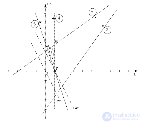
The scope of feasible solutions -  . The optimal solution is achieved in C (1.0) and w min = 6. This solution satisfies the first and second constraints as strict equalities (2-0 = 2> -6 and -4 + 0 = -4> -12). The corresponding variables of the direct problem are zero. Then
 3x 3 -x 4 = 6
x 3 = 12
From here x 3 = 12, x 4 = 30. Solution of the direct problem x 0 = (0,0,12,30). z max = 3 12-1 30 = 6. Since z max = w min = 6, the calculations are performed correctly.

Comments
To leave a comment
Mathematical methods of research operations. The theory of games and schedules.
Terms: Mathematical methods of research operations. The theory of games and schedules.