9 Algorithm for solving the transportation problem

The transport problem is solved by the method of potentials. Solve the problem with the transportation of grain. As an initial, we use the solution obtained by the northwest corner method.

In the method of potentials, each row i and each column j are assigned numbers, called potentials u _i and v _j . For each basic variable x _{ij, the} potentials must satisfy the equation:

u _i + v _j = c _ij

In our problem there are 7 unknown variables (potentials) and 6 equations corresponding to the basic variables. An arbitrary value is assigned to one of the potentials (u ₁ = 0 is usually assumed), and then the values ​​of the remaining potentials are calculated sequentially.

So, we have: u ₁ = 0, u ₂ = 5, u ₃ = 3

v ₁ = 10, v ₂ = 2, v ₃ = 4, v ₄ = 15.

Further, for each nonbasic variable, the quantities u _i + v _j -c _ij are calculated.

Since the minimum cost of transportation is sought, the variable that has the largest positive coefficient will be entered into the basis.

In this case, it will be x ₃₁ (9).

Calculations begin with the assignment u ₁ = 0. The v-potentials are then calculated for all columns that have basic variables in the first row. Further, on the basis of the equation of potentials corresponding to x ₂₂ , u _{2 is} determined. Knowing u _2, we calculate v ₃ and v ₄ , and finally u ₃ . The potentials are determined, then the quantities u _i + v _j -c _ij are calculated for each nonbasic variable x _ij .

We determined the variable x ₃₁ introduced into the basis. We must find the excluded.

Choosing x ₃₁ as the input variable, we want traffic on routes 3 - 1 to reduce the total cost of transportation. How much cargo can be transported on this route? Denote by the amount of cargo transported along the route (3.1), that is, x ₃₁ = . determine the conditions:

1. Restrictions on supply and demand must be met.

2. No route should be shipped with a negative volume.

Construct a loop that starts and ends in a cell (3.1). The cycle consists of consecutive horizontal and vertical segments connecting the cells corresponding to the current basis variables.

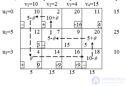
Find the value . In order to meet the supply-demand constraints, it is necessary to take and add alternately to the values ​​of variables located in the corner cells of the cycle. New values ​​of the basic variables will remain non-negative if the inequalities hold:

x ₁₁ = 5- ≥0

x ₂₂ = 5- ≥0

x ₃₄ = 10- ≥0

Hence it is clear that the greatest value = 5. x ₁₁ and x ₂₂ then vanish. You can exclude both x ₁₁ and and x ₂₂ . Exclude x ₁₁ .

So x ₃₁ = 5. Adjust the base variables in the corner cells.

The cost of transporting a unit of cargo decreased by u ₃ + v ₁ -c ₃₁ = 9 dollars, the total cost by 95 = 45 dollars.

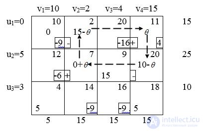
Repeat the calculation of potentials. The new variable entered will be x ₁₄ . From the loop x ₁₄ = 10, the excluded variable x ₂₄ .

New solution:

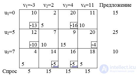
will be optimal, since u _i + v _j -c _{ij is} negative for all nonbasic variables.

In terms of the original problem, the solution makes sense:

The dual problem to the T-problem.

According to the general rule for the construction of dual tasks, the dual task for the transport one will be written as follows:

under restrictions:

u _i + v _i ≤c _ij ,,

The meaning of dual variables:

u _i ( ) - assessment of the unit of inventory (the potential of the i-th supplier);

v _j ( ) - assessment of the unit of demand (potential of the j-th supplier).

Assignment task

In practice, it is often necessary to solve the following tasks: distribute workers to workplaces so that the product manufacturing time is minimal, place sensors on objects so that information about the work of objects is maximum, distribute aircraft crews on flights so that LA downtime is minimal and etc.

The peculiarity of this task is that each resource (worker, sensor, crew) is used exactly once and one object is assigned to each object.

The solution of the problem is represented by a two-dimensional array or matrix x _ij , i = j = where m is the number of objects or resources. Desired variable

1, if the i-th resource is assigned to the j-th object,

x _ij =

0 otherwise.

The costs associated with assigning the i-th resource to the j-th object are denoted by the elements of the cost matrix c _ij . For any undesirable assignment, the corresponding value is assumed to be equal to a sufficiently large number M. The admissible solution of the problem is called assignment . In total, for a m × m matrix, there is m! making. A valid solution is built by selecting exactly one element in each row of the matrix x _ij and exactly one element in each of its columns.

Thus, the assignment problem is formulated as follows:

Z =

under restrictions:

a) each resource is used exactly once: for all i;

b) exactly one resource is assigned to each object: for all j.

Obviously, the assignment problem is a special case of the transport problem with single values ​​of the parameters a _i and b _i . To solve it, you can use any LP algorithm or potential method. But given its specificity, the so-called Hungarian method is used to solve it. It was first proposed by the Hungarian mathematician Egerwari in 1931. For a long time his work remained unknown. In 1953 The mathematician G. Kun translated the work of Egerwari into English, developed the ideas of Egerwari and called the method Hungarian. The Hungarian method was developed for manual calculations and is now of purely historical interest.

Example 1 Place 3 sensors in 3 objects in such a way that the cost of such placement is minimal. The cost matrix is:

Algorithm of the Hungarian method.

Stage 1. In the initial cost matrix, we define the minimum cost in each row and subtract it from the other elements of the row.

Stage 2. In the matrix obtained in the first stage, we find the minimum cost in each column and subtract it from the other elements of the column.

Stage 3. The optimal purpose will correspond to zero elements obtained in step 2.

Let p _i and q _{i be the} minimum values ​​in row i and column j, respectively.

p ₁ = 9, p ₂ = 9, p ₃ = 8

Subtract p _i from the elements of the corresponding rows.

q ₁ = 0, q ₂ = 2, q ₃ = 0.

Perform step 2.

Underlined zeros define the optimal solution. The cost of placement is equal to 9 + 10 + 8 = 27 USD Note that this amount is always equal to

(p ₁ + p ₂ + p ₃ ) + (q ₁ + q ₂ + q ₃ ).

Sometimes you can not immediately find a valid solution and need to resort to additional actions.

Example2.

p ₁ = 1, p ₂ = 7, p ₃ = 4, p ₄ = 5

q ₁ = 0, q ₂ = 0, q ₃ = 3, q ₄ = 0

It is impossible to assign 1 object for each sensor. It is necessary to add another step to the procedure of the Hungarian method.

Stage 2.1. If after completing the first and second stages no valid solution is obtained, perform the following actions:

1) In the last matrix hold the minimum number of horizontal and vertical straight lines in order to cross out all zero elements in the matrix.

2) Find the smallest not crossed out element and subtract it from the remaining not crossed out elements, and add to the elements standing at the intersection of straight lines.

3) If the new distribution does not allow finding a feasible solution, repeat step 2.1. Otherwise, go to step 3.

Underline the smallest element.

The optimal solution is underlined.

Z = 1 + 10 + 5 + 5 = 21 USD

The justification of the Hungarian method is based on the fact that if a number γ _i (= - p _i ) is added to each element of the i-th row, and a real number δ _j (= - q _j ) is added to each element of the j-th column, then minimization of the function equivalent to minimizing the function where d _ij = c _ij + γ _i + δ _i