Lecture
The tasks of the LP in many cases are called distribution type problems, the essence of which is as follows. Let the system under consideration be characterized by the presence of n types of activities for which there are various resources with numbers  . The possible volume of consumption of the i-th resource is limited by the non-negative value b i , and its consumption for the sale of a unit of product of the k-th activity is equal to a ik , where
  . In turn, the unit of the product of the k-th activity is characterized by the value of c k , called the specific profit (specific efficiency).
It is necessary to determine the volumes x k , activities of each type, which provide the maximum total income (efficiency) from the activities of the system without violating the restrictions imposed on the use of resources. In the general case, a distribution type problem has the form:


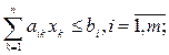 (2.3)
(2.3)

In order for an IO task to be presented as an LP task, the following conditions must be met:
- proportionality;
- additivity;
- non-negativity.
All of them took place when writing tasks (2.1, 2.2, 2.3).
In terms of distribution-type tasks, proportionality means that the costs of resources for any type of activity are proportional to the volume of production. Additivity indicates that the total amount of resources consumed by all types of activity is equal to the sum of resource expenditures for particular types of activity, and the total income from activities is equal to the sum of incomes from each of their types of activities. Non-negativity means that a negative output cannot be attributed to any of the activities.
In practice, the assumptions about proportionality and additivity in the construction of mathematical models of IO problems do not so often correspond to objective reality, therefore their acceptance in fact means approximation of a nonlinear linear model.
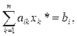
Consider a geometric method for solving problem (2.1). The basis of the method is a geometric (graphical) representation of the set of feasible solutions and the objective function.
The first stage of the graphical solution is to build a set of feasible solutions G.
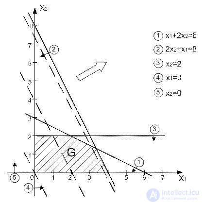
The second stage of the graphical solution consists in determining the direction of increase of the objective function f (x 1 , x 2 ) = 3x 1 + 2x 2 .
With an arbitrary fixed value  The equation f (x 1 , x 2 ) = f 0 can be represented as x 2 = -1.5x 1 + 0.5f 0 , this line is the line of the level of the objective function. To determine the direction of growth of the objective function (indicated by a sign), it suffices to depict the level lines f (x 1 , x 2 ) = f 01 and f (x 1 , x 2 ) = f 02 with f 01 02 . In order to find the optimal solution, one should move the level line in the direction of increasing the objective function until it moves to the region of inadmissible solutions R 2 \ G.
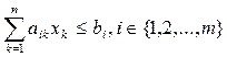
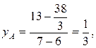
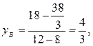
The figure shows that the maximum value of the objective function is reached at the vertex C of the polygon, which is the boundary G G of the set G of acceptable values. Since the point C is the intersection point of the lines x 1 + 2x 2 = 6 and 2x 1 + x 2 = 8, its coordinates x 1 * and x 2 * satisfy the system of these two equations. Therefore x 1 * = 10/3 and x 2 * = 4/3. In this case, the income will be maximum and equal  .
.
In this case, the specific profit from the products of each type with 1 = 3 and 2 = 2 is determined by the situation of the task (demand) and for uncontrollable reasons it can fluctuate within certain limits. Since the daily income
f (x 1 , x 2 ) = c 1 x 1 + c 2 x 2 ,
it is necessary to know the ranges of permissible values of specific profits that do not lead to new optimal solutions. From the figure it follows that for any positive values of c 1 and c 2 that satisfy the condition  the optimal solution is X * = (10/3; 4/3) T. In other cases, the solution will be different from that found. If, for example, f (x 1 , x 2 ) = 3x 1 + x 2 , then the optimal solution is (4; 0) T. With
  and
and  any point of the corresponding side of the polygon G G 1 , except for the point G 1 , determines the optimal solution.
It is also useful to know the decision maker about how the change in demand and change in the resources of the original products will affect the optimal solution. Such studies are called the analysis of the mathematical model (2.2) on sensitivity.
Let us turn to the problem of LP (2.3) of distribution type, assuming that the nonempty set G is bounded.
Let X * = (x 1 *, ..., x n *) T be the optimal solution of the LP problem of distribution type.
Limitation
 (2.4)
(2.4)
in problem (2.3) is called active if
and passive otherwise. If some restriction is active, then the corresponding resource is called deficient, since it is fully used when implementing the optimal solution. A resource corresponding to an inactive constraint is referred to as non-deficient resources (which are in some excess).
The graphic solution of the LP problem shows that the optimal solution can always be associated with at least one vertex of the polygon representing the set G of feasible solutions. Such a vertex is called the optimal vertex. Two optimal lines x 1 + 2x 2 = 6 and 2x 1 + x 2 = 8 pass through the optimal vertex G. Therefore, active are the restrictions on daily reserves of A and B.
When analyzing the sensitivity model, the right-hand sides of the constraints (2.4) determine:
a) the maximum allowable increase in the reserve of a scarce resource, which allows to obtain a new optimal solution, which in terms of the value of the objective function is more preferable than the old one;
b) the maximum allowable reduction in the stock of a non-deficient resource, which does not change the optimal solution found earlier.
It is clear that the analysis of the impact on the decision of an increase in the stock of a non-deficient resource (A) is limited to b 1 = 6. The figure shows that with an increase in the reserve b 1 of this resource, the straight line, defined by the equation x 1 + 2x 2 = b 1 , begins to move parallel to itself.
Until it passes through point F with b 1 = 7, this process corresponds to moving the optimal vertex C along the straight line given by the equation 2x 1 + x 2 = 8 in the direction of point F and increasing profit (the value of the objective function) at the optimal solution. When b 1 > 7, the analyzed resource is no longer scarce and a further increase in its stock loses its meaning. Note that for b 1 = 7, the optimal solution X * = (3 2) T corresponds to the value of the objective function f * = 13 and, along with the existing active constraint  another active limitation appears:
  .
.
A similar analysis can be carried out with respect to the second resource in short supply (initial product B), the consumption of which is limited to b 2 = 8. In Fig. 2.3 it can be seen that an increase in the stock b 2 of the initial product B makes sense up to the value b 2 = 12, at which the optimal solution X * = (6 0) corresponds to the value of the objective function f * = 18.
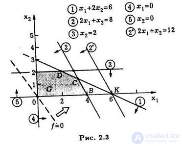
If there are restrictions on the costs associated with creating additional stocks of source products A and B, “it is important for the decision maker to know which resource should be preferred. For these purposes, an additional characteristic of the i-th resource in short supply is used - the value of the additional unit of the i-th resource, which is defined as the ratio of the maximum increment of the objective function to the maximum allowable increment of the volume of the i-th resource.
In this case, the value of the additional unit of the first resource (product A)
and the second resource (product B)
The results indicate that, if funds are available, additional investments should first be directed to increase the volume of product B, and only then to increase the volume of product A.
Forms of recording linear programming problems.
The standard form for recording LP tasks involves the fulfillment of two requirements:
1. All constraints (including non-negativity constraints of variables) are transformed into equalities with a non-negative right side.
2. All variables are non-negative.
Transformation of inequalities into equality.
Inequality of any type (  or
or  ) can be transformed into equality by adding to the left-hand side of inequalities additional variables — residual or redundant (balanced), which are associated with inequalities like “ "And" "Respectively.
For inequalities "", a non-negative residual variable is introduced in the left part of the inequality. For example, in the Reddy Mikks problem, the constraints on the quantity of raw materials M1 are given as inequality:
6x 1 + 4x 2 24
We introduce a new non-negative variable S 1 , which shows the remainder (unused quantity) of the raw material M1. This will lead to equality:
6x 1 + 4x 2 + S 1 = 24, S 1 0
Inequality type " "In LP tasks usually set the lower limit of something. The excess variable defines the excess of the left side above this boundary. So in the “diet” model, the inequality x 1 + x 2 0 indicates that the daily production of a dietary supplement must be at least 800 pounds. Mathematically, this is equivalent to:
x 1 + x 2 - S 1 = 800, S 1 0
A positive value of the redundant variable S 1 indicates the excess of production over the minimum value. Once again, we note that additional variables — residual S 1 and excess S 1 are always non-negative.
The right side of the inequality can always be made non-negative by multiplying the inequality -1. Inequalities converted to also by multiplying by -1. For example, inequality
-x 1 + x 2 -3
is equivalent to inequality:
-x 1 + x 2 + S 1 = -3, S 1 0
x 1 -x 2 -S 1 = 3.
Free variable
The condition of non-negativity of variables is natural. But situations are possible when variables can take on any valid values.
Example. The fast-food restaurant sells meat pies and hamburgers. A quarter of a pound of meat goes to a piece of cake, and 0.2 pounds on a hamburger. At the beginning of work there are 200 pounds of meat, you can get more, but with a premium of 25 cents. The remaining meat at the end of the day is donated to a charitable organization. Income from one pie 20 cents, from one hamburger, 15 cents. On the day the restaurant can not sell more than 900 servings. What should be the share of each dish to maximize income?

Comments
To leave a comment
Mathematical methods of research operations. The theory of games and schedules.
Terms: Mathematical methods of research operations. The theory of games and schedules.