4 Transition from graphic solution to algebraic. Algorithm simplex - method. Computational algorithm of the simplex method.

Limitations. Denote x ₁ and x ₂ respectively the number of servings of the pie and hamburgers. You can limit yourself to either 200 pounds of meat, or buy more. In the first case, the limit is 0.25x1 + 0.2x2,200, in the second, 0.25x1 + 0.2x2,200.

Naturally, the choice of inequality will influence the solution. Since we do not know what restriction is necessary, it is logical to replace them with one equality 0.25x ₁ + 0.2x ₂ -x ₃ = 200, where x _{3 is a} free variable. Here it plays the role of both excess and residual.

Objective function If you need to maximize income, you need to sell as much products as possible, then you need additional purchases of meat, in this case x ₃ should be negative, i.e. play the role of redundant variable. In order to uncover the “dual” nature of the variable x ₃ , let’s represent it as follows:

where 0

If a > 0 and , then the variable x ₃ plays the role of residual. If a > 0 and = 0, then x ₃ appears as redundant. So the restrictions now have the form

.

And the objective function

Z =

The transition from graphical solutions to algebraic.

The ideas underlying the graphic solution underlie the algebraic method, which is called the simplex method. In the graphical method, the solution space is defined as the intersection of half-spaces generated by constraints. In an algebraic or simplex method, the solution space is given by m linear equations and n non-negative variables.

In the algebraic representation, the number of equations m is always less than or equal to the number of variables n. (If the number of equations m is greater than the number of variables n, then mn equations are redundant.) If m = n and the system of equations is compatible, then it has one solution (if it is non-degenerate), if m

In the algebraic representation, candidates for the optimal solution (corner points in the graphical representation) are determined from a system of linear equations as follows. Let m

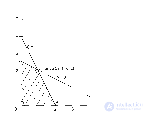
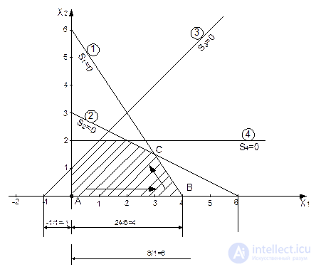
Example. Z = 2x ₁ + 3x ₂ max

2x ₁ + x ₂ four

x ₁ + 2x ₂ five

x ₁ x ₂ 0

After conversion to the standard form, we have the following LP problem.

Z = 2x ₁ + 3x ₂ max

2x ₁ + x ₂ + S ₁ = 4,

x ₁ + 2x ₂ + S ₂ = 5,

x ₁ , x ₂ , S ₁ , S ₂ 0.

We have a system of m = 2 equations for n = 4 variables. As we agreed, the corner points can be defined algebraically, assigning zero values ​​to n = m = 4-2 = 2 variables, and then solving the system for m = 2 variables. If we set x ₁ = 0 and x ₂ = 2 (point C).

Which variables are set equal to zero to get the corner points? You just need to consider all combinations of nm variables, equate them to zero and find all the corner points.

In our example, we have corner points. In the picture we see only 4. Where are the other two? In fact, points E and F are also corner points. But they are not yet candidates for an optimal solution, because they do not satisfy all restrictions.

To complete the transition to the algebraic method of solving the LP problem, it is necessary to somehow name the corner points of different types. The nm variables that are considered equal to zero are called non-basic variables. If the remaining m variables have a unique solution, they are called basic variables, and the set of solutions that they give constitute the basic solution. If all variables take non-negative values, this basic solution is called valid.

From this example, it is seen that as the dimension of the problem (n and m) increases, the process of enumerating all the corner points becomes a very difficult task. For example, when n = 20 and m = 10, you need to solve 184,756 systems of equations of the order of 1010. This is already an awesome computational problem. In reality, m and n can reach hundreds of thousands. Simplex method removes this problem.

Algorithm simplex - method.

So, the procedure of enumeration of all basic solutions is inefficient. Consider the simplex method.

The iterative nature of the simplex method.

Consider the solution space for the same example.

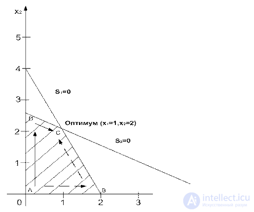
Usually, the simplex method algorithm starts from the starting point, where x ₁ = x ₂ = 0 (point A). At this starting point, the value of the objective function Z is zero. The question arises: if one or both of the nonbasic variables x ₁ and x ₂ take positive values, will this lead to an improvement in the objective function?

Z = 2x ₁ + 3x ₂ max.

Obviously, if the variable x ₁ and x ₂ (or both) take positive values, this will increase the value of the GF.

However, the algorithm of the simplex method at each step allows changing the value of only one nonbasic variable.

1. If you increase the value of the variable x ₁ , then its value should increase so as to correspond to the corner point B (candidates are only corner points). At point B, the simplex method should increase the value of the variable x ₂ , moving to the corner point C. Since point C corresponds to optimum, then the process ends. So simplex method algorithm creates path A B C.

2. If you first increase the value of the variable x ₂ , then the next corner point will be point D, from which we go to point C and end the process A D C.

Note that both ways are A B C and A D C are located along the boundary Γ of the solution space. So simplex - the method cannot immediately jump from t.A to t.C.

Does every nonbasic variable be made positive at a given corner point? If we consider the maximization problem, then we should choose a nonbasic variable that has the largest positive coefficient in the expression of the objective function. If there are several such variables, then the choice is arbitrary. This rule is empirical.

How to translate non-basic variables into basic variables and vice versa when moving from one corner point to another?

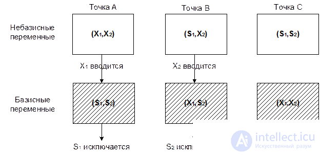
The figure shows that at point A, the variables S ₁ and S ₂ are basic, and the variables x ₁ and x ₂ are nonbasic If the variable x1 takes a positive value, we move to the corner point B, in which the state of the variable x ₁ changes from nonbasic to basic. At the same time, a variable that was basic at point A becomes nonbasic and takes a zero value at point B. Here it is significant, there is a simultaneous “state exchange” between nonbasic variable x ₁ and basic S ₁ , which leads to new basic (x ₁ , S ₂ ) and nonbasic (S ₁ , x ₂ ) variables at point B. At point A, variable x ₁ is introduced into the basic solution, and variable S _{1 is} excluded from the basic solution. In the terminology of the simplex method, the selected nonbasic (zero) variable is called input (to the basic solution), and the removed variable (from the basic solution) basic variable is excluded. In m. In the input and exclude variables will be respectively x ₂ and S ₂ .

Computational algorithm of the simplex method.

Consider the following example.

Let's return to the problem about the Reddy Mikks company. In standard form, this task is written as:

Z = 5x ₁ + 4x ₂ + 0S ₁ + 0S ₂ + 0S ₃ + 0S ₄ max

under restrictions:

6x ₁ + 4x ₂ + S ₁ = 24

x ₁ + 2x ₂ + S ₂ = 6

-x ₁ + x ₂ + S ₃ = 1

x ₂ + S ₄ = 2

x ₁ , x ₂ , S ₁ , S ₂ , S ₃ , S ₄ 0

Here S ₁ , S ₂ , S ₃ , S ₄ are additional (residual) variables.

The objective function will be represented as an equation:

Z - 5x ₁ - 4x ₂ = 0

The LP task in the standard form will be presented in the form of a table:

The table shows the sets of basic and nonbasic variables, as well as the solution corresponding to this (initial) iteration. The initial iteration starts from the point (x ₁ , x ₂ ) = (0,0). This corresponds to the following sets of basic and nonbasic variables:

Non-basic (zero): (x ₁ , x ₂ )

Basic: (S ₁ , S ₂ , S ₃ , S ₄ )

Since x ₁ = 0, x ₂ = 0 and the coefficients with the basic variables S ₁ , S ₂ , S ₃ , S ₄ in the equation of the objective function are zero, and in the formulas of the left parts of the equality of the restrictions - 1, without additional calculations we have: Z = 0, S ₁ = 24, S ₂ = 6, S ₃ = 1, S ₄ = 0.

In the table, the basic variables are listed in the left column “Basis”, and their values ​​in the right column “Solution”. Thus, the current corner point is defined.

Since the coefficient of the variable x1 in the formula of the objective function is the largest, it should be included in the number of base variables (it will be introduced). The table shows that the input variable is defined among the set of nonbasic as having the largest negative coefficient in the 2nd line. If all coefficients in the 2nd line are non-negative, then the maximum is reached.

To determine the excluded variable, it is necessary to calculate the intersection points of all functions with the positive direction of the x ₁ axis. These coordinates can be calculated as the ratio of the right-hand sides of the equality (the “Solution” column) and the coefficients of the variable x ₁ .

The maximum non-negative relation corresponds to the basic variable S ₂ , it is determined as excluded (that is, at the next iteration its value will be zero). The value of the input variable x _{1 is} also equal to the minimum non-negative relation: x ₁ = 6

Maximize

Z = 5x ₁ + 4x ₂

1) 6x ₁ + 4x ₂ + S ₁ = 24

2) x ₁ + 2x ₂ + S ₂ = 6

3) -x ₁ + x ₂ + S ₃ = 1

4) x ₂ + S ₄ = 2

x ₁ x ₂ 0

The value of the objective function will increase to 5. 4 = 20.

Replacing the excluded variable S ₁ with the input variable x ₁ leads to new sets of basic and non-basic variables and to a new solution in TV

Nonbasic (zero) variables (S ₁ , x ₂ )

Basic variables (x ₁ , S ₂ , S ₃ , S ₄ )

Now you need to perform the conversion in the table so that in the columns “Basis” and “Solution” you get a new solution corresponding to point B.

In the following table, which so far coincides with the initial, we define the leading column associated with the input variable and the leading row associated with the excluded variable. The element located at the intersection of the leading column and leading line is called leading.

Lead column

The process of calculating a new basic solution consists of two steps:

1. Calculate the elements of the new leading line.

New Sun = Current Sun / Lead

2. Calculation of the elements of the remaining lines, including the Z-line.

New line = Current line - its coefficient in the leading column New Sun

In the example, the calculations are:

1. New lead S ₁ line = Current lead S ₁ line / 6

2. New Z-line = Current Z-line - (-5) New Sun

3. New S ₂ line = Current S ₂ line - (1) New Sun

4. New S ₃ line = Current S ₃ line - (-1) New Sun

5. New S ₄ line = Current S ₄ line - (0) New Sun

Since the Z-line does not have negative coefficients corresponding to nonbasic variables S ₁ and S ₂ , the solution obtained is optimal.

The values ​​of the additional variables S ₁ = S ₂ = 0, S ₃ = 5/2 and S ₄ = 1/2 are consistent with the values ​​of the variables x ₁ and x ₂ .

With the help of the simplex table you can get a lot of additional information about the state of resources. The status “deficient” or “non-deficient” for a resource is determined by whether it is used or not. If the additional variable is zero, the resource is fully used, it receives the status of deficit.