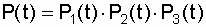
Lecture
7. Reliability of recoverable systems
7.1. Reliability of the recovered single-element system
7.2. Reliability of a non-redundant system with sequentially reconstructed elements
7.3. Reliability of the restored duplicated system
7. RELIABILITY OF RESTORABLE SYSTEMS
Sophisticated technical objects (systems), designed for a long service life, are usually created to be repaired. Section 2 gives an interpretation of the main indicators of reliability of the objects (elements) being restored: mean time to failure; bounce flow parameter; average recovery time; recovery rate; availability and operational readiness rates. This section discusses the methodology for analyzing the reliability of recoverable systems under various schemes for the inclusion of elements.
The transition of the system from an inoperative (limiting) state to a healthy state is carried out using recovery or repair operations. The first mainly include the operations of identifying a failure (determining its place and nature), replacement, regulation, and final operations of monitoring the health of the system as a whole. The transition of the system from the limit state to the operational state is carried out with the help of repair, at which the system resource in general is restored. Consider, for example, a vacuum switch. A vacuum chamber that cannot be repaired is replaced with a serviceable one if it fails, that is, the switch is restored to its working capacity by replacing the failed camera. If the same electromagnetic (or spring) drive switch fails, the switch can be restored by repairing the drive or replacing it with a serviceable one. In both cases, it is required to make adjustment of the drive and check the operation of the switch as a whole, by carrying out control operations "turn on" - "turn off".
7.1. Reliability of the recovered single-element system
In the analysis we use a number of the most frequently introduced assumptions.
 see 2.3.2.
  .
. 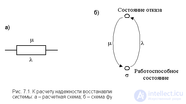
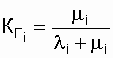
This system with an intensity of l tends to take a state of failure, and with an intensity of m , it goes into a healthy state.
In tab. 7.1 given the factory parameters l and m for high-voltage power equipment.
Table 7.1
Parameters l and m for some high-voltage devices
| Fault flow parameter l , 1 / year | Average recovery time  h h | ||
| Power transformer, U 1n = 110 kV |  | ||
|  | ||
|  | ||
| Disconnector, U n = 35 ... 220 kV | | ||
| | ||
| |
Denote the stable state of the system indices:
1 - failure, that is, the system is in a state of recovery with a recovery rate of m = const;
0 - healthy state with a fault flow parameter
w = const, w = l .
For the analyzed system, taking into account the accepted assumptions, four types of transition from the state at the moment of time t to the state at the moment of time (t + D t) are possible :
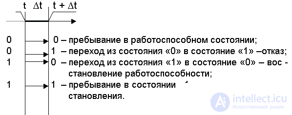
These transitions can be represented as a transition graph of the system states with restoration (Fig. 7.2).
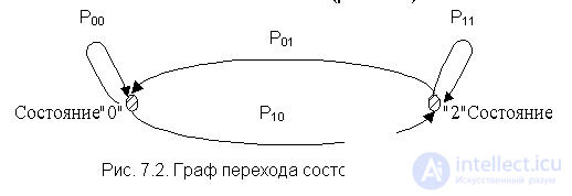
The state transition graph [13] corresponds to a 2 x 2 transition probability matrix:
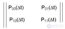 (7.1)
(7.1)
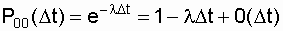
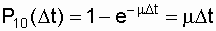
The diagonal elements of this matrix are respectively defined as the probability of failure-free operation on the interval D t:
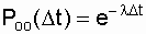
and the probability of continuing to restore the system on the segment D t:
 .
.
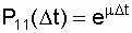
We use the formula for the decomposition of the function  in row [11]:
 .
.
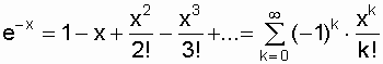
In highly reliable elements l <  1 / h, then when decomposing the function R 00 ( D t) into a series , while maintaining high accuracy of the calculation, it is possible to limit oneself only to the first two terms of the series. Let l =
  1 / hour, D t = 1 hour, then
 .
.

Thus, we write
 .
.
Respectively
 .
.
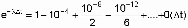
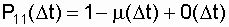
From the properties of the matrix it follows that the sum of the elements of each row of the matrix is equal to one, as the sum of the probabilities of the occurrence of incompatible components of the full group of events [13], from which it follows
P 00 ( D t) + P 01 ( D t) = 1; Р 01 = 1 - Р 00 ( D t) = l D t + 0 ( D t);
Р 11 ( D t) + Р 10 ( D t) = 1; Р 10 = 1 - Р 11 ( D t) = m D t + 0 ( D t).
To compile the equations of the probabilities of the states of the system, write the formula of the total probability for each column of the matrix [11, 13, 21]
 - for the first column;
 - for the second column,
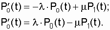
where P 0 (t) is the probability of the system being in the zero (healthy) state at the moment of time t; P 1 (t) is the probability of the system being in the "1" state (failure) at time t.
Use the record of the derivative of the function f (x):
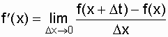
and by analogy with this expression for our case we write:
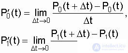
In these expressions, we substitute the open formulas for the total probabilities  and
and  , we make the appropriate transformations and get a system of two differential equations with respect to the probabilities of the system being in the "0" and "1" states:
 (7.2)
(7.2)
Under initial conditions, P 0 (t = 0) = 1; Р 1 (t = 0) = 0, at the initial moment of time (t = 0) the recoverable system is operational - is in the state "0". Solving differential equations gives
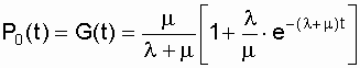 . (7.3)
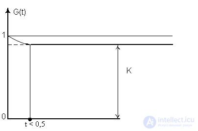
The probability of the operational state of the system at time t is a function of readiness G (t). The readiness function is the probability of the operational state of the system being restored at a certain point in time t. This indicator is a comprehensive indicator of reliability, evaluating the two properties of the system - reliability and maintainability. Note that G (t) does not give an estimate for the entire period from 0 to t, but only at a given moment of time t, because before that the system could be both in a healthy (0) and inoperable (1) states.
In fig. 7.3 plotted: 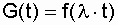 at
at  .
.

Assuming l = const, you can clearly see how the reliability of the system will increase by increasing m (reducing the recovery time  ) for a specific time t. For example, if you increase m tenfold for the moment lH t = 1, the reliability will increase from
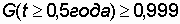
G (t) = 0.41 to G (t) = 0.95. For highly reliable systems, for example, a transformer, when: l <  1 / h, m >
  1 / h, it is advisable to determine the reliability rating for the year of operation. In this case, it is convenient to use the availability factor.
Define the limit value G (t) by the expression (7.3):
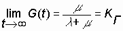 . (7.4)
Asymptotic value of the readiness function at t (r) Ґ is the availability factor.
Thus, the availability factor represents the probability that the system will be operational at an arbitrary point in time, except for planned periods during which the use of the system for its intended purpose is not foreseen.
Example. There is a recoverable system with a failure flow parameter l =  1 / h = const, average recovery rate
  1 / h Determine how much the reliability of this system will increase due to the higher organization of the work of the repair personnel, if the system recovery intensity has doubled (the recovery time has been halved).
Decision.  h;
h;  50 h. The system availability factor to improve the organization of labor of repair personnel was
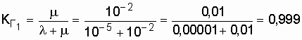 .
.
With improved work organization
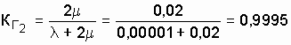 .
.
The sum of the costs associated with improving the organization of labor and the economic effect of increasing reliability (improving maintainability), we can conclude about the feasibility of this method of improving the reliability of the system.
7.2. Reliability of a non-redundant system with sequentially reconstructed elements
A system consisting of N consecutive recoverable elements fails when any of the system elements fails. The simplest failure and recovery flows are assumed.  . As shown in [15, 19], with given assumptions and known values of the availability factors of each of the series-connected elements
  , the system availability ratio is determined by the expression
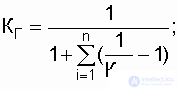
and accordingly, given  ,
, 
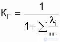 .
.
Example. The recoverable system consists of three elements connected in series with reliability parameters:  = 0.6;
  = 0.8;
  = 0.7. It is known that
  .
.
Determine the reliability factor.
Decision. Substituting the specified values of availability factors in the expression of the KG system, we get
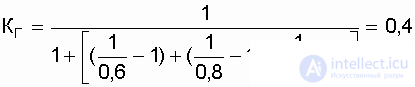 .
.
We also note here that in computational practice, the probability formula for the failure-free operation of an unrepairable system with the main combination of elements is often used when
 .
.
In this case  that, as we see, is associated with a gross error. The product of the probabilities of failure-free operation of elements of an unrepairable system is a mathematical assessment of the fact that the operational state of the three elements constituting the system of non-recoverable elements coincides, that is, the operational state of the system. The product of the availability factors of the repaired elements does not reflect the fact that the operating states of the elements coincide [19].
7.3. Reliability of the restored duplicated system
Consider a system for which reliability duplication is used: the same system is added in parallel to the main system. In both systems (chains), the parameters of the failure flows are the same, l = const, the same picture for the restoration flow, that is, m = const. Such a duplicate system can be in three states:
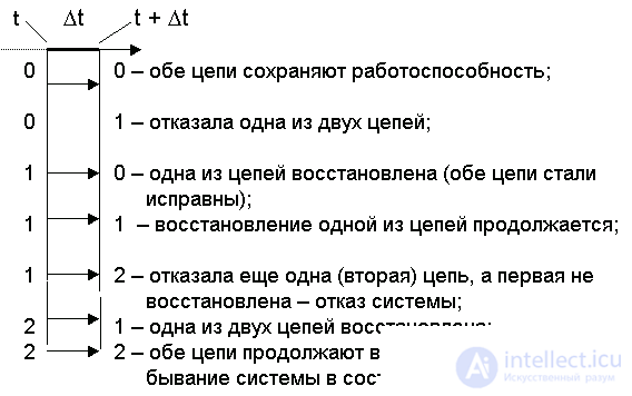
"0" - both systems (circuits) are operational;
"1" - one chain is restored, the other is operational;
"2" - both chains are restored. From the point of view of performing functional tasks assigned to the system, the state "2" corresponds to a failure. This system has seven types of transition from the state at the moment of time t to the state at the moment of time t + D t:
The indicated transitions are shown in Fig. 7.5 as a state transition graph.
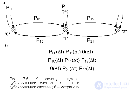
The transition graph corresponds to the transition probability matrix.  . Extreme elements of the secondary diagonal of the matrix have order 0 ( D t), since, according to the initial assumption, the flow of failures in the system is the simplest, and the recovery time is distributed exponentially. According to the simplest flow, the situation in the first row of the matrix is eliminated, when during the time D t the system can go from the state "0" to the state "2", Р 02 ( D t) = 0. Arguing the same way, we write P 20 ( D t) = 0. With the simplest flow, the system can go from state “0” with probability P 01 ( D t) to state “1” or with probability P 00 ( D t) in state “0”. Exactly the same picture corresponds to the state "2". With a probability of P 21 ( D t), the system can go to the state "1" (one circuit will recover) or with a probability P 22 ( D t) it will remain in the state "2" (both circuits are inoperative - a failure state). The elements of the first row of the matrix of transition probabilities depend on the mode of use of the backup chain. So with a loaded reserve operating in both circuits, the intensity of the flow of failures is 2 l , and when not loaded - l (the unloaded circuit is always ready for operation and does not change its characteristics, l = const). therefore
 , (7.6)
where y is the coefficient taking into account the state of the reserve (y = 0 when unloaded mode and y = 1 when loaded).
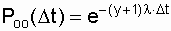
Using the expansion of a power function in a series, taking into account the approximation of the sum of the dropped members of the series to zero, we write
P 00 ( D t) = 1 - (y + 1) HlЧD t. (7.7)
Given that for the first row of the matrix
Р 00 ( D t) + Р 01 ( D t) = 1,
will get
P 01 ( D t) = 1 - P 00 ( D t) = (y + 1) H lЧD t. (7.8)
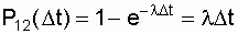
The elements of the second row of the matrix of transition probabilities (7.5), respectively, are written as:
Р 10 ( D t) + Р 11 ( D t) + Р 12 ( D t) = 1;
 , (7.9)
 , (7.10)
 . (7.11)
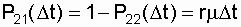
The elements of the third row of the analyzed matrix, taking into account the number of repair crews and the repeated restoration of the failed circuits, are accordingly defined as:
R 21 ( D t) + R 22 ( D t) = 1;
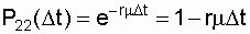 ; (7.12)
 , (7.13)
where r is the number of repair teams (r = 1 or r = 2).
When duplicating with recovery, there are six possible tasks for analyzing the reliability of such a system:
1) a system with a loaded reserve to the first failure (y = 1, r = 0);
2) a system with an unloaded reserve to the first failure (y = 0, r = 0);
3) repeatedly restored system with a loaded reserve and one repair team (y = 1, r = 1);
4) a repeatedly restored system with a loaded reserve and two repair crews (y = 1, r = 2);
5) repeatedly restored system with unloaded reserve and two repair crews (y = 1, r = 2);
6) a repeatedly restored system with an unloaded reserve and one repair crew (y = 0, r = 1).
To determine P 0 (t), P 1 (t), 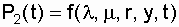 it is necessary to compose and solve a system of three differential equations
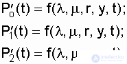 (7.14)
Where  - constant coefficients.
To do this, based on the properties of the columns of the matrix, it is necessary to write the expressions of the formulas for the total probabilities P 0 (t + D t), P 1 (t + D t), P 2 (t + D t), then write the derivatives for the expressions of the probabilities of the system in the states "0", "1", "2" and reduce them to a system of equations:
 (7.15)
The formulas for the total probabilities are written on the basis of the matrix (7.5), respectively:
on the first column 
on the second column  ;
;
по третьему столбцу  .
.
Подставив в эти выражения соответствующие значения переходных вероятностей, получим систему из трех дифференциальных уравнений (7.15) с четырьмя постоянными коэффициентами l , m , r, у.
Определение искомых вероятностей пребывания системы в состояниях "0", "1" и "2" в момент времени t производится при следующих начальных условиях: Р 0 (t = 0) = 1; Р 1 (t = 0) = 0; Р 2 (t = 0) = 0, то есть система первоначально включается в работу с обоими исправными цепями. Решение системы (7.15) подробно изложено в специальной литературе, например в [13]. Искомое выражение функции готовности анализируемой системы при найденных значениях Р 0 (t), Р 1 (t), Р 2 (t) на основе известного свойства 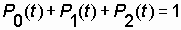 удобнее записать в виде:
 .
.
Анализируемая система получается высоконадежной. Даже в нерезервированной восстанавливаемой системе при 
 , и значение этой функции быстро приближается к коэффициенту готовности. В связи со сказанным, оценку надежности ответственных систем, рассчитанных на длительный срок эксплуатации, целесообразно производить с помощью коэффициента готовности.
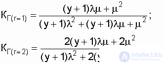
Используя данные [13], запишем коэффициенты готовности дублированной системы с многократным восстановлением с одной (r = 1) и двумя (r = 2) ремонтными бригадами:
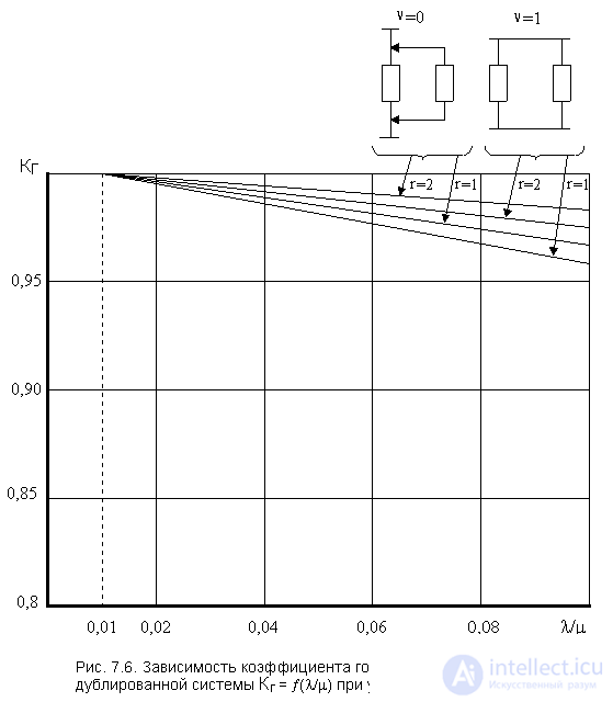
In fig. 7.6 представлены графики коэффициента готовности  для различных схем использования резерва и количества ремонтных бригад.
Из графика видно, что введение резервирования в восстанавливаемую систему дает существенное приращение надежности системы при относительно невысокой надежности основной цепи. К примеру, при  заметен прирост надежности даже при введении второй ремонтной бригады (r = 2). Но по мере роста надежности исходных цепей эффект от введения второй бригады снижается, а при
  на графике уже невозможно увидеть различия значений коэффициента готовности не только при изменении количества ремонтных бригад, но и при переходе со схемы нагруженного дублирования к дублированию замещением. Так при
  отношение значения коэффициента готовности схемы дублированной замещением к значению коэффициента готовности схемы нагруженного дублирования, при одной ремонтной бригаде в обоих вариантах равно
 =1,0001.
Например, в высоковольтной электроустановке с показателями безотказности и ремонтопригодности Т = 20000 ч, t в =100 ч ( 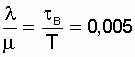 ), использование схемы нагруженного дублирования повышает надежность установки до
  а при дублировании замещением до
  .
.
Таким образом, при относительно высоком уровне надежности исходной системы (схемы) выигрыш в надежности при переводе схемы с режима у = 1 на режим у = 0 ощутимого результата не дает. При эксплуатации, например двухтрансформаторной подстанции, когда средняя интенсивность отказов (параметр потока отказов) одной трансформаторной цепи l < 0,2 1/год, интенсивность восстановления m > 0,01 1/ч, (  ) схема включения резервного трансформатора подстанции (нагруженное дублирование или дублирование замещением) должна определяться по фактическому значению потери мощности в трансформаторах, а не по уровню надежности. Как известно, потеря мощности в трансформаторе
 ,
,
где  - потеря мощности в магнитной системе (в стали магнитопровода) трансформатора и от нагрузки не зависит;
  - потеря мощности в меди (алюминии) обмоток трансформатора и зависит от квадрата тока.
Выбирать необходимо такую схему включения трансформаторов, которая связана с меньшей потерей мощности. Если подстанция имеет в течение суток нагрузку то высокую, то низкую в четко выраженные интервалы времени, то возникает экономическая целесообразность часто изменять схему включения трансформаторов. Расчеты показывают, что в современных трансформаторах напряжением 35; 10,5; 6,3 кВ и мощностью до 10 тыс. кВА, при нагрузке подстанции, превышающей 0,7 мощности одного трансформатора, экономически выгодно переходить на схему нагруженного дублирования (режим у = 1). Для обеспечения такого режима работы подстанции необходимы циклостойкие выключатели (например вакуумные), способные переключаться под рабочей нагрузкой тысячи раз [14]. Это особенно характерно для подстанций, где преобладает коммунально-бытовая нагрузка, при которой ярко выражены часы максимальной нагрузки (обычно с 7.00 до 9.00 и с 18.00 до 21.00 часа местного времени). В оставшееся время суток нагрузка многократно снижается, и тогда выгодно включать только один трансформатор (режим у = 0). В связи с этим следует отметить, что в установках, где часто меняется нагрузка в широком диапазоне особо эффективны будут тиристорные выключатели рабочих токов, у которых нет технических ограничений по количеству операций (циклов) "включить"-"отключить".
Такие высоковольтные восстанавливаемые дублированные установки, как кабельные линии и воздушные линии электропередачи должны работать по схеме нагруженного дублирования. При этом, как это было показано выше, достигается экономический эффект от снижения потери энергии, и сохраняется высокая надежность электропередачи.
7.4. Надежность восстанавливаемой системы при различных способах резервирования элементов
При решении задач обеспечения надежности сложных систем, состоящих из ряда звеньев, когда каждое звено может иметь свою, отличную от соседних, схему включения резерва, процедура расчетов многократно усложняется.
В системах электроснабжения задача усложняется от того, что в каждом из звеньев, например в трансформаторной подстанции, применяются секционирующие выключатели, образующие "мостиковые" схемы. В результате реальная система имеет такую структуру соединения или взаимодействия элементов, которая не может быть сведена ни к параллельно-последовательной, ни к последовательно-параллельной схеме. Методы оценки различных показателей надежности сложной системы весьма специфичны и чисто аналитический расчет на основе вероятностных моделей, изложенных выше, практически неприемлем.
Для решения задач надежности в сложных системах используются такие методы как логико-вероятностный расчет с помощью дерева отказов, таблично-логический метод расчета, экспертно-факторный анализ надежности [8, 9, 10, 11, 21].

Comments
To leave a comment
Theory of Reliability
Terms: Theory of Reliability