Lecture
3. MAIN MATHEMATICAL MODELS MOST FREQUENTLY USED IN RELIABILITY CALCULATIONS
3.1. Weibull distribution
The experience of operating many electronic devices and a significant amount of electromechanical equipment shows that they are characterized by three types of dependences of the failure rate on time (Fig. 3.1), corresponding to the three periods of life of these devices [3, 8, 10, 19].
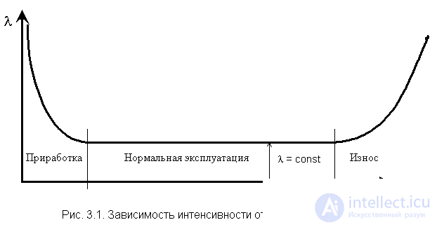
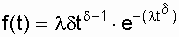
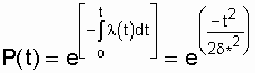
It is easy to see that this drawing is similar to fig. 2.3, since the graph of the function l (t) corresponds to the Weibull law. These three types of dependences of the failure rate on time can be obtained by using the two-parameter Weibull distribution for a probabilistic description of random time between failures [12, 13, 15]. According to this distribution, the probability density of the moment of failure
 , (3.1)
where d is a form parameter (determined by selection as a result of processing experimental data, d > 0); l is the scale parameter
 .
. The failure rate is determined by the expression
 (3.2)
(3.2)
Probability of uptime

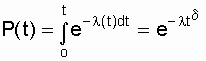 , (3.3)
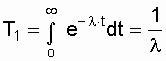
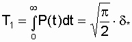
and the average time to failure
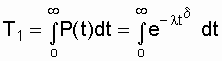 . (3.4)
Note that with the parameter d = 1, the Weibull distribution becomes exponential, and with d = 2 it becomes the Rayleigh distribution.
When d < 1, the failure rate monotonously decreases (the period of running-in), and when  monotonously increases (wear period), see fig. 3.1. Consequently, by selecting the parameter d, it is possible to obtain, at each of the three sections, such a theoretical curve l (t), which is close enough to the experimental curve, and then the calculation of the required reliability indices can be made on the basis of a known regularity.
The Weibull distribution is close enough for a number of mechanical objects (for example, ball bearings), it can be used for accelerated testing of objects in the forced mode [12].
3.2. Exponential distribution
As noted in subsection. 3.1 The exponential distribution of the probability of failure-free operation is a special case of the Weibull distribution, when the form parameter d = 1. This distribution is one-parameter, that is, one parameter l = const is enough to write the calculated expression . The reverse statement is true for this law: if the failure rate is constant, then the probability of failure-free operation as a function of time obeys the exponential law:
 . (3.5)
The average uptime with an exponential distribution law of the uptime interval is expressed by the formula:
 . (3.6)
 . (3.7)
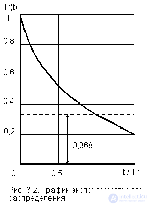
 Note that the probability of failure-free operation on an interval exceeding the average time T 1 , with an exponential distribution will be less than 0.368:
P (T 1 ) =  = 0.368 (Fig. 3.2).
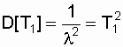
The duration of the normal operation period before the onset of aging may be significantly less than T 1 , that is, the time interval at which the use of the exponential model is permissible is often less than the average uptime calculated for this model. This is easily justified by taking advantage of the variance of uptime. As is known [4, 13], if for a random variable t the probability density f (t) is given and the mean value (expectation) T 1 is determined, then the variance of the uptime can be found by the expression:
 (3.8)
(3.8)
and for the exponential distribution, respectively:
 . (3.9)
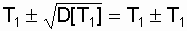
After some transformations we get:
 . (3.10)
 , that is, in the range from t = 0 to t = 2T 1 . As you can see, the object can work and a small period of time and time.
 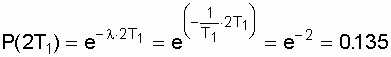 .
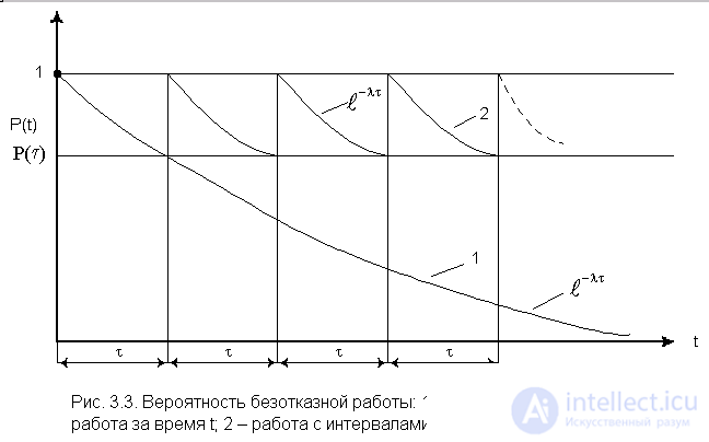
. It is important to note that if the object has worked, suppose that time t without failure, retaining l = const, then the further distribution of the uptime will be the same as at the time of the first activation l = const.
Thus, disabling a healthy object at the end of an interval  and its new inclusion on the same interval many times will lead to a saw-tooth curve
  (see fig. 3.3).
Other distributions do not have the specified property. At first glance, a paradoxical conclusion follows: since the device does not age for all time (does not change its properties), it is not advisable to carry out the prevention or replacement of devices to prevent sudden failures obeying an exponential law. Of course, this conclusion does not contain any paradox, since the assumption of an exponential distribution of the uptime interval means that the device does not age. On the other hand, it is obvious that the longer the time for which the device is turned on, the more all sorts of random reasons that can cause a device to fail. This is very important for the operation of devices when it is necessary to choose intervals at which preventive work should be carried out in order to maintain high reliability of the device. This question is considered in detail in [1].
The exponential distribution model is often used for a priori analysis, since it allows using simple calculations to obtain simple relationships for different variants of the system being created. At the stage of a posteriori analysis (experimental data), the compliance of the exponential model with the test results should be checked. In particular, if, when processing the test results, it turns out that 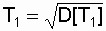 then this is proof of the exponentiality of the dependency being analyzed.
In practice, it often happens that l№ const, however, in this case it can be used for limited periods of time. This assumption is justified by the fact that for a limited period of time, the variable failure rate without a large error can be replaced by [12, 15] with the average value:
l (t) " l cp (t) = const.
3.3. Rayleigh distribution
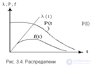
The probability density in the Rayleigh law (see. Fig. 3.4) has the following form
| 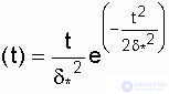 , (3.11)
where d * is the Rayleigh distribution parameter (equal to the mode of this distribution [13]). It does not need to be confused with the standard deviation:
 .
. 
The failure rate is equal to:
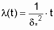 .
.
A characteristic sign of the Rayleigh distribution is a straight line of the graph l (t), starting from the origin.
The probability of failure-free operation of the object in this case is determined by the expression
 . (3.12)
Mean time to failure
 . (3.13)
3.4. Normal distribution (Gaussian distribution)
The normal distribution law is characterized by the probability density of the species.
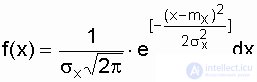 , (3.14)
where m x , s x are the mean and the standard deviation of the random variable x , respectively.
When analyzing the reliability of electrical installations in the form of a random variable, in addition to time, the values of current, voltage and other arguments often appear. The normal law is a two-parameter law for which you need to know m x and s x .
The probability of failure-free operation is determined by the formula
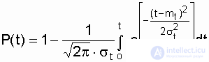 , (3.15)
and the failure rate - according to the formula
 .
.
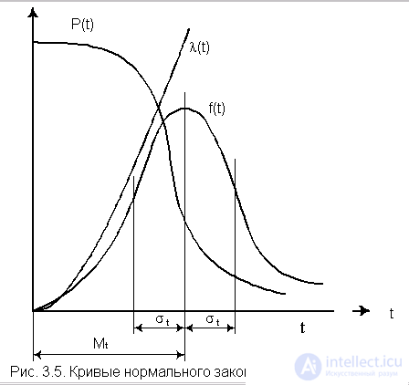
In fig. 3.5 shows the curves l (t), P (t) and ¦ (t) for the case of s t << m t characteristic of the elements used in automatic control systems [3].
This tutorial shows only the most common laws for the distribution of a random variable. A number of laws are also known, which are also used in reliability calculations [4, 9, 11, 13, 15, 21]: gamma distribution,  -distribution, distribution of Maxwell, Erlang, etc.
It should be noted that if the inequality s t << m t is not observed, then a truncated normal distribution should be used [19].
For a reasonable choice of the type of practical distribution of time to failure, you need a large number of failures with an explanation of the physical processes occurring in the objects before failure.
In highly reliable elements of electrical installations, during operation or tests for reliability, only a small fraction of the initially existing facilities fails. Therefore, the value of numerical characteristics found as a result of the processing of experimental data strongly depends on the type of expected time to failure distribution. As shown in [13,15], with different laws of time to failure, the values of the average time to failure, calculated from the same source data, can differ hundreds of times. Therefore, it is necessary to pay special attention to the choice of the theoretical model of the distribution of uptime to failure, with appropriate evidence for approximating the theoretical and experimental distributions (see Section 8).
3.5. Examples of using distribution laws in reliability calculations
Let us determine the reliability indices for the most frequently used laws of the distribution of the time of failure occurrence.
3.5.1. Determination of reliability indicators with the exponential distribution law
An example . Let an object have an exponential distribution of the time of occurrence of failures with a failure rate of l = 2.5 × 10 –5 1 / h.
It is required to calculate the main indicators of the reliability of a non-recoverable object for t = 2000 h.
Decision.

 .
.  h
h 3.5.2. Determining Reliability Indicators for Rayleigh Distribution
Example. Distribution parameter d * = 100 h.
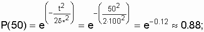
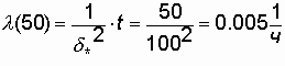
It is required to determine for t = 50 h the values of P (t), Q (t), l (t), T 1 .
Decision.
Using the formulas (3.11), (3.12), (3.13), we get
 ;
;
 ;
;

3.5.3. Definition of circuit parameters in Gaussian distribution
Example. The electrical circuit is assembled from three series-connected type resistors:  ;
;
 (in% the value of resistance deviation from the nominal value is set).
It is required to determine the total resistance of the circuit taking into account the deviations of the resistor parameters.
Decision.
It is known that in mass production of the same type of elements, the density of distribution of their parameters obeys the normal law [15]. Using the rule of 3 s (three sigma), we define the ranges in which the values of the resistances of the resistors lie:  ;
; 
 Consequently,
When the values of the parameters of the elements have a distribution, and the elements are randomly selected when creating the scheme, the resulting value of R e is a functional variable, also distributed according to the normal law [12, 15], with the variance of the resulting value, in our case  determined by the expression
 .
.
Since the resulting value of R e distributed according to the normal law, then, using the rule of 3 s , we write
 ,
,
Where  - nominal passport parameters of resistors.

In this way
 , или
, или
 .
.
Данный пример показывает, что при увеличении количества последовательно соединенных элементов результирующая погрешность уменьшается. В частности, если суммарная погрешность всех отдельных элементов равна ± 600 Ом, то суммарная результирующая погрешность равна ± 374 Ом. В более сложных схемах, например в коле***тельных контурах, состоящих из индуктивностей и емкостей, отклонение индуктивности или емкости от заданных параметров сопряжено с изменением резонансной частоты, и возможный диапазон ее изменения можно предусмотреть методом, аналогичным с расчетом резисторов [15].
3.5.4. Пример определения показателей надежности неремонтируемого объекта по опытным данным
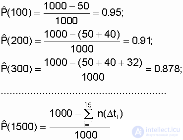
Пример. На испытании находилось N о = 1000 образцов однотипной невосстанавливаемой аппаратуры, отказы фиксировались через каждые 100 часов.
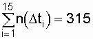
Требуется определить  в интервале времени от 0 до 1500 часов. Число отказов
  на соответствующем интервале
  представлено в табл. 3.1.
| Номер i-го интервала |  ,ч ,ч |  PC. PC. |  |  ,1/ч ,1/ч |
 | ||||
 |
Решение.
Согласно формуле (2.1) для любого отрезка времени, отсчитываемого от t = 0,
 , - по формуле Гаусса

где t i - время от начала испытаний до момента, когда зафиксировано n(t i ) отказов.
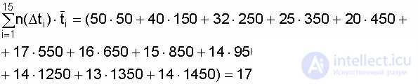
Подставляя исходные данные из табл. 3.1, получим:
Воспользовавшись формулой (2.9), получим значение , 1/ч:
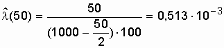 ;
;
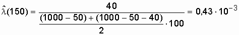 ;
;
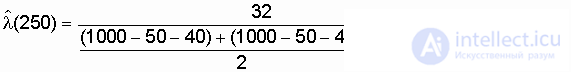 ;
;
.................................................................................................................
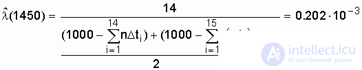 .
.
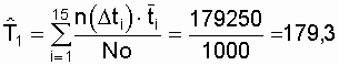
Средняя наработка до отказа, при условии отказов всех N o объектов, определяется по выражению
 ,
,
 объектов. Поэтому по полученным опытным данным можно найти только приближенное значение средней наработки до отказа. В соответствии с поставленной задачей воспользуемся формулой из [13]:
 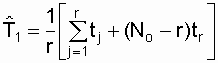 при r Ј N о , (3.16)
 где tj - наработка до отказа j-го объекта ( j принимает значения
от 1 до r); r - количество зафиксированных отказов (в нашем случае r = 315); tr - наработка до r-го (последнего) отказа.
Полагаем, что последний отказ зафиксирован в момент окончания эксперимента (tr = 1500).
На основе экспериментальных данных суммарная наработка объектов до отказа равна
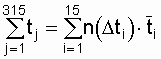 ,
,
где  - среднее время наработки до отказа объектов, отказавших на интервале .
В результате
 ч.
ч.
Примечание: обоснование расчетов  , по ограниченному объему опытных данных, изложено в разд. eight.
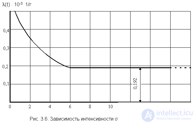
По полученным данным (см. табл. 3.1) построим график l (t).
Из графика видно, что после периода приработки t і 600 ч интенсивность отказов приобретает постоянную величину. Если предположить, что и в дальнейшем l будет постоянной, то период нормальной эксплуатации связан с экспоненциальной моделью наработки до отказа испытанного типа объектов. Тогда средняя наработка до отказа
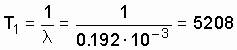 ч.
ч.
Таким образом, из двух оценок средней наработки до отказа  = 3831 ч и T 1 = 5208 ч надо выбрать ту, которая более соответствует фактическому распределению отказов. В данном случае можно предполагать, что если бы провести испытания до отказа всех объектов, то есть r = N о , достроить график рис. 3.6 и выявить время, когда l начнет увеличиваться, то для интервала нормальной эксплуатации ( l = const) следует брать среднюю наработку до отказа T 1 = 5208 ч.
В заключение по данному примеру отметим, что определение средней наработки до отказа по формуле (2.7), когда r << N о , дает грубую ошибку. В нашем примере
 ч.
ч.
If instead of N о we put the number of failed objects
r = 315, then we get
 h
h
In the latter case, the objects that failed in the test time in the amount of N о - r = 1000-315 = 685 pcs. In general, they did not get into the assessment, that is, the mean time to failure was determined only by 315 objects. These errors are quite common in practical calculations.

Comments
To leave a comment
Theory of Reliability
Terms: Theory of Reliability