Lecture
6. RELIABILITY OF NON-RECOVERABLE RESERVED SYSTEMS
In the operation of systems, there is a widespread method of increasing their reliability by introducing additional elements into the system diagram, which can work in parallel with the main elements or be connected to the place of the failed element. Thus, a backup system is a system in which a failure occurs only after the failure of any main element and all of the reserve elements of the element being analyzed. The most common backup methods are shown in Fig. 6.1.
With a general reservation, the main object (system) is reserved as a whole, and if it is separate, separate parts (elements) of the system are reserved. Under the multiplicity of redundancy "m" refers to the ratio of the number of backup objects to the number of primary. When reserving with integer multiplicity, the value of m is an integer (for example, if m = 2, then there are two reserve objects for one main object). When reserving fractional multiplicity, a fractional non-convertible number is obtained. For example, when m = 4/2, the reserve objects are 4, the main 2, the total number of objects is 6. It is impossible to reduce the fraction, since the new ratio will reflect a completely different physical meaning.
By the method of inclusion, the reservation is divided into permanent and reservation by replacement. With a permanent backup, the backup objects are connected to the load continuously throughout the operation time and are in the same conditions as the main objects. When reserving with a replacement, the main objects (connected to the load) are replaced after their failure.
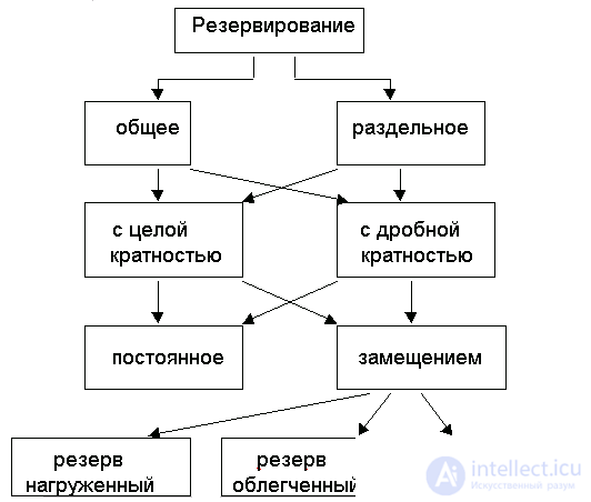
Fig. 6.1. Reservation methods
6.1. General reservation with always-on reserve and with full multiplicity
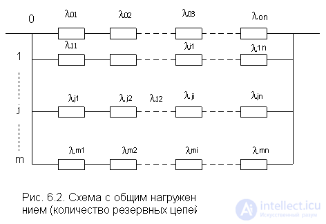
The reserved scheme is shown in fig. 6.2.
This scheme resembles the main "0" electrical circuit with "n" series-connected elements. In parallel, it includes "m" backup circuits with exactly the same parameters of the elements as in the main circuit.
The analysis will be performed under the following assumptions:
1) element failures are random and independent events;
2) switching devices are ideal (their reliability is P (t) = 1, and the main and backup circuits are equally reliable);
3) repair of the redundant system is excluded.
Based on the accepted assumptions, using the formula (4.1) for the main and backup circuits, we determine the probability of failure-free operation
 , (6.1)
Where  - probability of failure-free operation of the i-th element of the main "0" chain;
  - probability of failure-free operation of the i-th element of the j-th
Since all elements of the same name in each chain have the same parameters and are in the same conditions, their reliability at the same time t is the same. Therefore, for all circuits
 . (6.2)
The probability of failure of the analyzed circuits, respectively, will be recorded
 . (6.3)
We clarify the concept of system failure. It will fail if the main circuit and all backups fail. Mathematically, this state is written accordingly:
 (6.4)
(6.4)
where Q o (t) is the probability of failure of the main circuit.
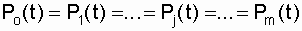
Since all circuits are identical and are in the same conditions,

and then the probability of system failure
 . (6.5)
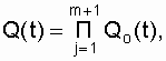
Using the expression (6.3), we write
 (6.6)
(6.6)
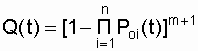 . (6.7)
The redundant system can be in one of two incompatible states — operational, when at least one of the circuits is operational, and failure, when all m + 1 circuits have failed. Therefore, mathematically it looks like this:
P (t) + Q (t) = 1.
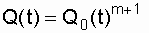
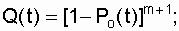
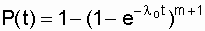
As a result, we find that the probability of system failure with the number of chains m + 1 is equal to
Р (t) = 1 - Q (t);  . (6.8)
In the case when  = const, in each of the chains (the simplest flow of failures) expression
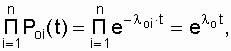
Where 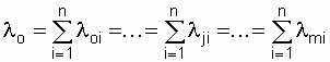 . (6.9)
Then instead of the expression (6.8) we write
 , (6.10)
Where 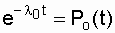 - probability of failure-free operation of the main circuit.
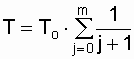
Mean time to failure of the redundant system
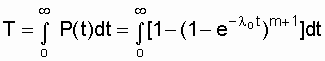 .
.
After some transformations [13, 15] we get
 ;
;  . (6.11)
The failure rate of the system, as is known, is determined by the expression
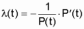 .
.
For a more visual representation of the gain in reliability with the use of a common loaded redundancy with integer multiplicity, we construct a graph (Fig. 6.3) of the dependence
 . (6.12)
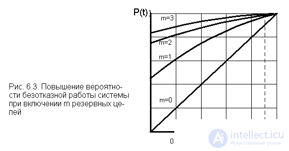
From pic. 6.3 it can be seen that if P o (t) has a small value, for example, P o (t) < 0.8, then for m> 2 one can see a significant increase in reliability and. However, with an increase in the reliability of the main circuit P о (t), the efficiency of using several backup branches decreases sharply. If the reliability of the main circuit P о (t) > 0.95, then a significant increase in P (t) is noticeable when only one backup circuit is turned on. The power supply industry uses elements of high reliability, the average time to failure of which is often more than 10 years, and the cost of the facilities is considerable. In this regard, as a rule, it is more profitable to hold a series of events that will allow to raise the P o (t) of the main object (single-circuit power lines, cable lines, single-transformer substations, etc.) to more than 0.95 without significant costs then, in order to raise the reliability of the redundant system to the required level, it is possible to do with only one backup chain with a level of reliability, as in the main circuit.
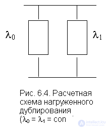
6.2. System reliability with load duplication
The method of loaded duplication is a special case of the general loaded redundancy with a whole multiplicity, m = 1, that is, one backup chain falls under one main circuit under load. In fig. 6.4 (the calculated reliability scheme is shown).
Probability of system failure-free operation according to the formula (6.10)
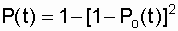 , (6.13)
where Р о (t) is the probability of failure-free operation of the main circuit ( 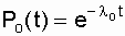 ).
).
The average time to failure of the system is determined by the expression (6.11):
 .
.
Determine the dependence of the failure rate of the system from time to time:
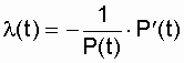 . (6.14)
Substitute the expression (6.13) and its derivative into expression (6.14). After some simplifications we get:
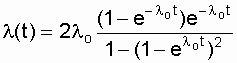 . (6.15)
To construct the graph l (t) (Fig. 6.5), we define the limiting values of this function:
 ;
; 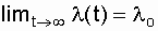 .
.
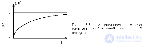
The figure shows that the failure rate of the system increases over time. This suggests that with a large t, the probability of failure of one of the circuits is high, and the system can go into single-element operation mode l = l 0 . Note also the initial stage (when t " 0). This system has a very high reliability ( l (t) (r) 0).
In fig. 6.6 shows the graph of the function P (t), constructed from the dependence (6.13). There is also a graph of P o (t) of the main circuit (without a reserve).
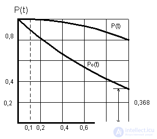
Fig. 6.6. Dependence of the probability of failure-free operation of the main circuit P 0 (t) and the system of two elements P (t) from l 0 t
 1 / year, t = 0.5 years (
  ), the value of P (t = 0.5) > 0.999.
 This level of reliability of power supply to a wide range of consumers is often sufficient. In [1], it is described how, due to maintenance, a high level of reliability of non-repairable systems operating according to the method of loaded duplication is achieved for a considerable time.
In conclusion, it should be noted that if the duplicated non-repairable system is turned on for a considerable period without maintenance, then the level of system reliability will be unacceptably low.

Comments
To leave a comment
Theory of Reliability
Terms: Theory of Reliability