6.2 Functional points method (function points) - performance measurement

This method is used to measure performance instead of the outdated linear approach, where performance was measured by the number of lines of program code. Functional points (function points) were first proposed by IBM employee Alan Albrecht in 1979 [58].

The advantage of this method is that since the application of functional points is based on the study of requirements, the assessment of the necessary labor costs can be performed at the earliest stages of work on the project. To support and develop this method in 1986, the International Function Point User Group (IFPUG) was created.

The method is as follows.

First, the functions of the developed software are highlighted, and at the user level, rather than the program code. For example, consider a software package that implements various methods for sorting one-dimensional arrays. One of the functions of the user of this complex will be the choice of the method, and we will describe it as an example [61].

The next step of the method will be to count the number of factors listed below:

• external inputs. Only those inputs that have a different effect on the function differ. The function method selection has one external input;

• external exits. Different outputs are considered for different algorithms. Imagine that our function generates a message - a text description of the selected method, and calls another function that directly implements the selected sorting algorithm, therefore, it has two outputs;

• external requests. In our example there are none;

• internal logical files — a data group that is created or maintained by a function is considered to be one. As an internal logical file for our function, we take a text file containing descriptions of the algorithms;

• external logical files - user data located in files external to this function. Each data group is taken as a unit. External to our function is the file with the result of processing.

Further, the obtained values ​​are multiplied by the coefficients of complexity for each factor (according to 1РР1Ю) and summed to obtain the full size of the software product. The values ​​of these coefficients are given in table. 9.1.

Table 9.1. The values ​​of the coefficients of complexity

Parameter	Simply	Average	Complicated
External inputs	3	four	6
External outputs	four	five	7
External requests	3	four	6
Internal logical files	7	ten	15
External logical files	five	7	ten

For the example we are considering, we take the values ​​given in table. 9.2.

The size of our function will be:

FR = 1x3 + 1x4 + 1x5 + 1x7 + 1x7 = 26.

This number is a preliminary estimate and needs to be clarified.

Table 9.2. Example of complexity factors

Parameter	Simply		Average		Complicated
	Koliche property	Coef ficient	Koliche property	Coef ficient	Koliche property	Coef ficient
External inputs	one	3	0	four	0	6
External outputs	one	four	one	five	0	7
External requests	0	3	0	four	0	6
Internal logical files	one	7	0	ten	0	15
External logical files	0	five	one	7	0	ten

The next step in determining the size of the program code by the method of function points is to assign a weight (from 0 to 5) to each characteristic of the project. We list these characteristics:

1. Is data backup required?

2. Need data sharing?

3. Are used distributed computing?

4. Is performance important?

5. Does the program run on heavily loaded hardware?

6. Is prompt data entry required?

7. Are many data entry forms used?

8. Are database fields updated promptly?

9. Input, output, queries are complicated?

10. Is internal computation difficult?

11. The code is intended for reuse?

12. Is data conversion and program installation required?

13. Need a lot of installations in different organizations?

14. Need to maintain customization and ease of use?

Values ​​for these characteristics are defined as follows: 0 - never; 1 - sometimes; 2 - rarely; 3 - medium; 4 - often; 5 - always.

These characteristics for an example of the function are summarized in Table. 9.3.

Table 9.3. Example of project characteristics

Characteristic	Value in the example	Characteristic	Value in the example
one	3	eight	0
2	one	9	3
3	0	ten	four
four	four	eleven	five
five	2	12	0
6	one	13	0
7	3	14	3

Determined by 5 - the sum of all weights.

Finally, the refined functional size is calculated by the formula

UVR = FR X (0.65 + 0.01 X 5). (9.3)

The refined functional size of the function method selection will be as follows:

UVR = 26 x (0.65 + 0.01 x 29) = 17.19.

The resulting result shows that the function of the method selection is quite simple and does not require large labor costs. The resulting values ​​are then used to estimate the cost of the project.

Currently, there are several modifications of the functional point method [57].

Property points

If the above characteristics do not reflect the true complexity of implementation (for example, when developing operating systems), instead of the method of functional points, use its improved version proposed by 1988 by Kuipers Jones, the method of properties points. This method corrects the estimates obtained by the method of functional points taking into account the algorithmic complexity of the software product.

Mark II method

The Mark II method was introduced by Charles Simons also in 1988. This method is more suitable for evaluating complex systems than the classical function point method. It allows one to achieve the same result both when evaluating the system as a whole, and when summing up the estimates obtained for the subsystems that comprise it.

Three-dimensional functional points

In 1991, the software division of Boeing Corporation proposed another solution - the method of three-dimensional functional points. The difference from the classical method is that the complexity of the software product is estimated in three directions - data, functions and control. The advantage of the method is its applicability not only to the evaluation of software projects, but also to the assessment of the complexity of tasks in other areas of activity.

Object points

The object point method adapts the original method of the function points to an object-oriented programming technology.

Function point method overview

Functional point analysis is a standard method for measuring the size of a software product from the point of view of system users. The method developed by Alan Albrecht (Alan Albrecht) in the mid-70s. The method was first published in 1979. In 1986, the International Function Point User Group (IFPUG) was formed, which published several revisions of the method [2].

The method is intended for estimating, based on a logical model, the volume of a software product by the amount of functionality requested by the customer and supplied by the developer. The undoubted advantage of the method is that the measurements do not depend on the technological platform on which the product will be developed, and it provides a uniform approach to the evaluation of all projects in the company.

When analyzing by the method of functional points, the following sequence of steps should be performed (Figure 37):

1. Determination of type of assessment.
2. Determining the scope and boundaries of the product.
3. Counting function points associated with the data.
4. Calculation of function points associated with transactions.
5. Determination of the total number of non-aligned functional points (UFP).
6. Determining the value of the equalization factor (FAV).
7. The calculation of the number of aligned functional points (AFP).

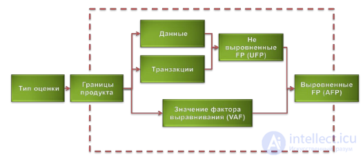
Figure 37. Function point analysis procedure

Determination of type of assessment

The first thing to do is to determine the type of assessment to be performed. The method provides estimates of three types:

1. Development project. Estimated amount of functionality delivered to users in the first release of the product.
2. Development project Evaluated at the functional points of the draft revision: add, change and delete functionality.
3. Product. Estimated volume of existing and installed product.

Determining the scope and boundaries of the product

The second step is to define the scope and boundaries of the product. Depending on the type, the area of ​​assessment may include:

• All developed features (for development project)
• All add, change, and delete functions (for support projects)
• Only the functions actually used, or all the functions (in evaluating the product and / or products).

The third step. The boundaries of the product (Figure 38) determine:

• What is "external" in relation to the product being evaluated.
• Where is the "border system" through which the transactions are transmitted or received by the product, from the point of view of the user.
• What data is supported by the application, and what - external.

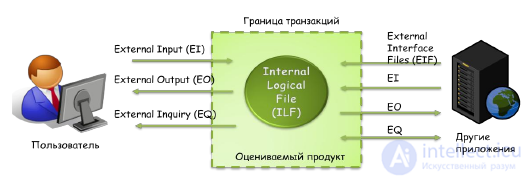
Figure 38. Product boundaries in the function point method

The logical data of the system are:

• Internal logical files (ILFs) are user-defined logically related data groups or blocks of control information that are supported within the product.
• External Interface Files (EIFs) are user-defined logically related data groups or blocks of management information that are referenced by a product but supported outside the product.

An example of logical data (information objects) can be: a client, an account, a tariff plan, a service.

Counting the function points associated with the data

The third step is to count the function points associated with the data. First, the complexity of the data is determined by the following indicators:

• DET (data element type) - non-repeatable unique data field, for example, Customer Name - 1 DET; Client's address (postal code, country, region, district, city, street, house, building, apartment) - 9 DET's
• RET (record element type) - logical data group, for example, address, passport, phone number.

Estimation of the number of non-aligned functional points depends on the complexity of the data, which is determined on the basis of the complexity matrix (Table 7).

Table 7. Data complexity matrix

	1-19 DET	20-50 DET	50+ DET
1 RET	Low	Low	Average
2-5 RET	Low	Average	High
6+ RET	Average	High	High

Evaluation of data in non-aligned functional points (UFP) is calculated differently for internal logical files (ILFs) and for external interface files (EIFs) (Table 8) depending on their complexity.

Table 8. Data evaluation in non-aligned functional points (UFP) for internal logical files (ILFs) and external interface files (EIFs)

Data complexity	The number of UFP (ILF)	Number of UFP (EIF)
Low	7	five
Average	ten	7
High	15	ten

For illustration, consider an example of evaluation at non-aligned functional points of the “Customer” data object (Figure 39).

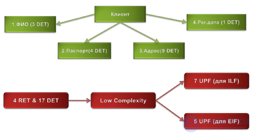
Figure 39. An example of evaluation in non-aligned functional points of the “Client” data object.

The “Client” object contains four logical data groups, which together consist of 15 non-repeatable unique data fields. According to the matrix (Table 7), we should estimate the complexity of this data object as “Low”. Now, if the object being evaluated belongs to internal logical files, then according to Table 8, its complexity will be 7 unaligned function points (UPF). If the object is an external interface file, then its complexity will be 5 UPF.

Calculation of function points associated with transactions

The counting of functional points associated with transactions is the fourth step of the analysis using the functional point method.

A transaction is an elementary indivisible closed process that represents a value for a user and translates a product from one consistent state to another.

The method distinguishes the following types of transactions (Table 9):

• EI (external inputs) - external input transactions, an elementary operation to process data or control information that enters the system from outside.
• EO (external outputs) - external output transactions, an elementary operation to generate data or control information that goes beyond the system. Assumes a certain logic of processing or computing information from one or more ILFs.
• EQ (external inquiries) is an external request, an elementary operation that, in response to an external request, retrieves data or control information from the ILF or EIF.

Table 9. The main differences between the types of transactions. Legend: O - basic; D - additional; NA - not applicable.

Function	Transaction type
	EI	Eo	EQ
Changes system behavior	ABOUT	D	NA
Support one or more ILF	ABOUT	D	NA
Presentation of information to the user	D	ABOUT	ABOUT

The assessment of transaction complexity is based on the following characteristics:

• FTR (file type referenced) - allows you to count the number of different files (information objects) such as ILF and / or EIF modified or readable in a transaction.
• DET (data element type) - a unique unique data field. Examples EI: input field, button. EO: report data field, error message. EQ: input field for search, output field for search result.

To assess the complexity of transactions are matrices that are presented in Table 10 and Table 11.

Table 10. The matrix of complexity of external input transactions (EI)

EI	1-4 DET	5-15 DET	16+ DET
0-1 FTR	Low	Low	Average
2 FTR	Low	Average	High
3+ FTR	Average	High	High

Table 11. The matrix of complexity of external output transactions and external requests (EO & EQ)

EO & EQ	1-5 DET	6-19 DET	20+ DET
0-1 FTR	Low	Low	Average
2-3 FTR	Low	Average	High
4+ FTR	Average	High	High

Evaluation of transactions in non-aligned functional points (UFP) can be obtained from the matrix (Table 12)

Table 12. The complexity of transactions in non-aligned functional points (UFP)

Transaction complexity	Number of UFP (EI & EQ)	Number of UFP (EO)
Low	3	four
Average	four	five
High	6	7

As an example, consider the evaluation of the control transaction (EI) for a dialog box that sets spelling check parameters in MS Office Outlook (Figure 40).

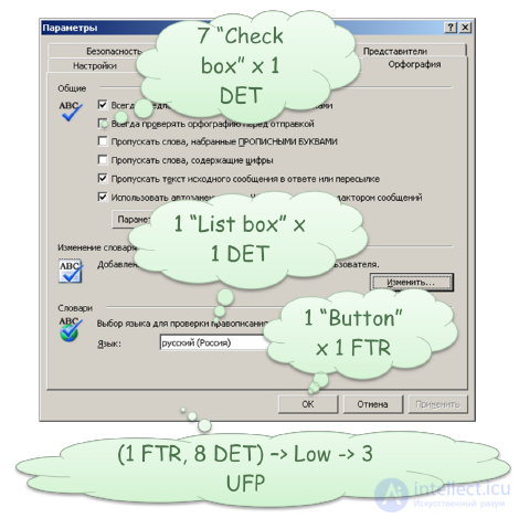
Figure 40. Dialog box controlling spell checking in MS Office Outlook

Each "Check box" is rated as 1 DET. Dropdown list - 1 DET. Each control button should be treated as a separate transaction. For example, if we evaluate the control transaction using the “OK” button, then for this transaction we have 1 FTR and 8 DET. Therefore, according to the matrix (Table 10), we can estimate the complexity of the transaction as Low. And, finally, in accordance with the matrix (Table 12), this transaction should be evaluated in 3 non-aligned functional points (UFP).

Determination of the total number of non-aligned functional points (UFP)

The total volume of the product in non-aligned functional points (UFP) is determined by summing over all information objects (ILF, EIF) and elementary operations (EI, EO, EQ transactions).

Determination of the equalization factor (FAV) value

In addition to the functional requirements for the product, system-wide requirements are imposed that limit developers to choose a solution and increase the complexity of development. The leveling factor (VAF) is applied to account for this complexity. The value of the factor VAF depends on 14 parameters that determine the system characteristics of the product:

1. Data exchange (0 - the product is a standalone application; 5 - the product communicates using more than one telecommunication protocol).
2. Distributed data processing (0 - the product does not move data; 5 - distributed data processing is performed by several components of the system).
3. Performance (0 - no user performance requirements are set; 5 - response time is strongly limited critical for all business operations, to meet the requirements, special design solutions and analysis tools are needed.
4. Restrictions on hardware resources (0 - no restrictions; 5 - the entire product must function on a specific processor and cannot be distributed).
5. Transactional load (0 - not a lot of transactions, no peaks; 5 - the number of transactions is large and uneven, special solutions and tools are required).
6. User interaction intensity (0 - all transactions are processed in batch mode; 5 - more than 30% of transactions are interactive).
7. Ergonomics (end-user efficiency) (0 - no special requirements; 5 - performance requirements are very stringent).
8. The intensity of data changes (ILF) by users (0 - not required; 5 - changes intensive, strict requirements for restoration).
9. Processing complexity (0 - processing is minimal; 5 - security requirements, logical and mathematical complexity, multithreading).
10. Reuse (0 - not required; 5 - the product is developed as a standard reusable component).
11. Easy installation (0 - no requirements; 5 - installation and software update is performed automatically).
12. Ease of administration (0 - not required; 5 - the system automatically restores itself).
13. Portability (0 - the product has only 1 installation on a single processor; 5 - the system is distributed and assumes installation on various hardware and operating systems).
14. Flexibility (0 - not required; 5 - flexible query system and the construction of arbitrary reports, the data model is changed by the user in an interactive mode).

14 system parameters (degree of influence, DI) are evaluated on a scale from 0 to 5. The calculation of the total effect of 14 system characteristics (total degree of influence, TDI) is carried out by simple summation:

TDI = ∑ DI

The value of the equalization factor is calculated by the formula

VAF = (TDI * 0.01) + 0.65

Например, если, каждый из 14 системных параметров получил оценку 3, то их суммарный эффект составит TDI = 3 * 14 = 42. В этом случае значение фактора выравнивания будет: VAF = (42 * 0.01) + 0.65 = 1.07

Расчет количества вьровненных функциональных точек (AFP)

Дальнейшая оценка в выровненных функциональных точках зависит от типа оценки. Начальное оценка количества выровненных функциональных точек для программного приложения определяется по следующей формуле:

AFP = UFP * VAF.

Она учитывает только новую функциональностсть, которая реализуется в продукте. Проект разработки продукта оценивается в DFP (development functional point) по формуле:

DFP = (UFP + CFP) * VAF,

где CFP (conversion functional point) — функциональные точки, подсчитанные для дополнительной функциональности, которая потребуется при установке продукта, например, миграции данных.

Проект доработки и совершенствования продукта оценивается в EFP (enhancement functional point) по формуле:

EFP = (ADD + CHGA + CFP) * VAFA + (DEL* VAFB),

Where

• ADD — функциональные точки для добавленной функциональности;
• CHGA — функциональные точки для измененных функций, рассчитанные после модификации;
• VAFA — величина фактора выравнивания рассчитанного после завершения проекта;
• DEL — объем удаленной функциональности;
• VAFB — величина фактора выравнивания рассчитанного до начала проекта.

Суммарное влияние процедуры выравнивания лежит в пределах ±35% относительно объема рассчитанного в UFP.

Метод анализа функциональных точек ничего не говорит о трудоемкости разработки оцененного продукта. Вопрос решается просто, если компания разработчик имеет собственную статистику трудозатрат на реализацию функциональных точек. Если такой статистики нет, то для оценки трудоемкости и сроков проекта можно использовать метод COCOMO II.