The use of classical neural networks for image recognition is complicated, as a rule, by a large dimension of the vector of the input values of the neural network, a large number of neurons in the intermediate layers and, as a result, large expenditures of computing resources for training and computing the network. Convolutional neural networks are less likely to have the disadvantages described above.
The convolutional neural network (
pers .
Convolutional neural network ,
CNN ) is a special architecture of artificial neural networks proposed by Jan Lecun and aimed at effective image recognition and is part of the technology of deep learning (eng.
Deep leaning ). This technology is built by analogy with the principles of the visual cortex, in which so-called simple cells were discovered, which respond to straight lines from different angles and complex cells, the reaction of which is associated with the activation of a specific set of simple cells. Thus, the idea of convolutional neural networks is the alternation of convolutional layers (English
convolution layers ) and sub-sampling layers (English
subsampling layers , subsample layers). [6]
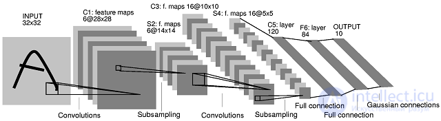
Figure 1. The architecture of the convolutional neural network
The key point in the understanding of convolutional neural networks is the concept of so-called “shared” weights, i.e. a part of the neurons of some considered layer of the neural network may use the same weights. Neurons using the same weights are combined into
feature maps , and each neuron of the feature map is associated with a portion of the neurons of the previous layer. When calculating the network, it turns out that each neuron performs convolution (the operation of convolution) of a certain area of the previous layer (determined by the set of neurons associated with the neuron). The layers of a neural network constructed in the manner described are called convolutional layers. In addition, convolutional layers in a convolutional neural network can be subsampling layers (performing the functions of reducing the dimension of the feature map space) and fully connected layers (the output layer, as a rule, is always fully connected). All three types of layers can alternate in random order, which allows to draw feature maps from feature maps, which in practice means the ability to recognize complex feature hierarchies [3].
What exactly affects the quality of pattern recognition when training convolutional neural networks? Puzzled by this question, stumbled upon an article by Matthew Zeiler (
Matthew Zeiler ). He developed the concept and technology of
Deconvolutional Neural Networks (
DNN ) for understanding and analyzing the performance of calibration neural networks. The article by Matthew Ziler offers
Deconvolutional Neural Network s technology, which builds hierarchical representations of the image (Figure 2), taking into account filters and parameters obtained during
CNN training (Figure 2). These representations can be used to solve problems of primary signal processing, such as noise reduction, and they can also provide low-level functions for object recognition. Each hierarchy level can form more complex functions based on the functions of the levels located in the hierarchy below.
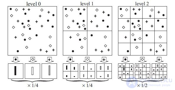
Figure 2. Image views
The main difference between
CNN and
DNN is that in
CNN the input signal is subjected to several layers of convolution and subsampling.
DNN, on the contrary, seeks to generate an input signal in the form of a sum of convolutions of feature maps taking into account the applied filters (Fig. 3). To solve this problem, a wide range of tools of the pattern recognition theory is used, for example, algorithms for eliminating blur (
deblurring ). The work, written by Matthew Zyler, is an attempt to link the recognition of image objects with low-level tasks and data processing and filtering algorithms.
Understanding the convolution operation requires an interpretation of the behavior of feature maps in intermediate layers. To study a convolutional neural network, a
DNN is attached to each of its layers, as shown in Figure 3, providing a continuous path from the network's outputs to the image's input pixels. First, a convolution operation is performed on the input image and feature maps are calculated over all layers, then, to study the behavior in
CNN , weights of all neurons in the layer are set to zero and the resulting feature maps are used as input parameters for the attached deconvnet layer. Then we successively carry out the operations: (I) separation, (II) rectification and (III) filtration. The trait maps in the layer below are reconstructed in such a way as to obtain the necessary parameters, such as the neuron weights in the layer and the filters used. This operation is repeated until the values of the input pixels of the image are reached.
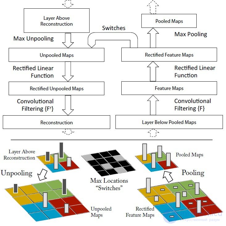
Figure 3. The process of research of convolutional neural networks using
DNN The separation operation: in convolutional neural networks, this is a union operation, it is irreversible, however, an approximate inverse value can be obtained by recording the location of the maxima within each region. The operation of unification is understood as the summation of all input values of the neuron and the transfer of the obtained sum to the transfer function of the neuron. In
DNN , the disconnect operation uses changes in the set of variables placed in the layer above, at the appropriate places in the layer that is being processed at the moment (see Figure 2).
Rectification operation: a convolutional neural network uses a non-linear function (
relu (x) = max (x, 0) , where the x-input image is), ensuring that the resulting feature maps will always be positive.
Filtering operation: a convolutional neural network uses the filters obtained in the network training process to convolve the feature maps from the previous layer. To understand which filters were applied to an image, deconvnet uses transposed versions of the same filters. Designing a “descent down” from higher levels uses parameter changes derived from
CNN training. Since these changes are characteristic of this input image, the reconstruction obtained from one function thus resembles a small piece of the initial image with structures (Fig. 4) weighted in accordance with their contribution to the feature map. Since the model is trained in accordance with the identified features, they, the structures, implicitly show which parts of the input image (or parts of two different images) are different in the features obtained [4]. Also, the resulting structures allow conclusions to be drawn about which low-level features of the image are key to its classification.

Fig. 4. Image structures.
Although in theory the global minimum can always be found, in practice it is difficult. This is due to the fact that the elements in the feature maps are connected to each other through filters. One element in the map can affect other elements that are located far from this element, which means that minimization can take a very long time.
Benefits of using
DNN :
1) conceptually simple training schemes.
DNN training is carried out through the use of unpooling, rectification and image filtering, as well as feature maps obtained during
CNN training;
2) applying
DNN to source images, you can get a large set of filters that cover the entire image structure using primitive representations; In this way, filters are obtained that apply to the entire image, and not to each small piece of the original image. This is a great advantage, as there is a more complete understanding of the processes that occur during
CNN training.
3) views (Fig. 2) can be obtained without configuring special parameters or additional modules, such as separation, rectification and filtering. They, representations, turn out in the course of training of
CNN ;
4) the
DNN approach is based on the global minimum search method, as well as the use of filters obtained from
CNN training, and is designed to minimize ill-conditioned costs that arise in the convolutional approach.
The review article also contains the results of experiments conducted by Matthew Zyler. The network proposed by him at
ImageNet 2013 competitions showed the best result in solving the problem of image classification, the error was only 14.8%. Classification of objects in 1000 categories. The training sample consisted of 1.2 million images, and the test sample of 150 thousand images. For each test image, the recognition algorithm should issue 5 class marks in descending order of their reliability. When calculating the error, it was taken into account whether the most reliable mark corresponds to the mark of the class of the object actually present in the image, which is known for each image. The use of 5 tags is intended to exclude the “punishment” for the algorithm in the case when it recognizes objects of other classes in the image, which can be implicitly represented [1]. More competitions for ImageNet 2013 are described here.
The results of
Deconvolution Neural Networks are shown in Figure 5.
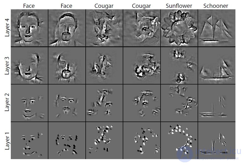
Figure 5.
DNN results
Seiler further plans to develop
DNN technology in the following areas:
1) Improving the classification of images in
DNN. DNN networks have been introduced in order to understand the features of the learning process of convolutional networks. Using the parameters obtained during the training of the convolutional neural network, in addition to the high-level functions, a mechanism can be provided to increase the level of classification in
DNN . Further work is related to the classification of the original images, so you can say that the template method will be applied. Images will be classified based on the class to which the object belongs.
2) scaling
DNN . Inference methods used in
DNN , by their nature, are slow, since many iterations are necessary. Numerical approximation methods based on direct communication should also be investigated. This will require only those functions and merge parameters for the current batch of snapshots that allow the
DNN to scale to large data sets.
3) improvement of convolutional models for the detection of several objects in the image. Convolutional networks are known to be used for classification for many years and they have recently been applied to very large data sets. However, further development of algorithms used in the convolutional approach is necessary to detect several objects at once in the image. To detect
CNN at once several objects in the image, a large set of training data is required, and the number of parameters for training the neural network also increases significantly. [4]
After studying his article, they decided to conduct a study on
DNN . Matthew Seiler developed the
Deconvolutional Network Toolbox for
Matlab . And immediately ran into a problem - the non-trivial task of installing this
Toolbox . After a successful installation, we decided to share these skills with habravchanami.
So, let's proceed to the installation process.
Deconvolutional Network Toolbox was installed on a computer with the following technical characteristics:
•
Windows 7 64x •
Matlab b2014a Let's start with preparing the software that needs to be installed:
1)
Windows SDK , during installation it is necessary to remove the check marks from the
Visual C ++ Compilers items
Microsoft Visual C ++ 2010 If the computer already has
VS 2010
redistributable x64 or
VS 2010
redistributable x86
installed , you will have to remove it.
Finish the installation of the
Windows SDK , and install the patch
2) After that, download and install
VS 2010
3) Also, to install this toolbox, you need to install the
icc compiler, in our case it is the
Intel C ++ Composer XE Compiler 2011 .
4) In
Matlab, type the command
mbuild -setup
and automatically select
SDK 7.1 .
Similarly happens with
mex –setup
If the compiler was successfully installed, then you can now start building the toolbox.
Software preparation is complete. Getting to the compilation process.
1) Download toolbox with
www.matthewzeiler.com/software/DeconvNetToolbox/DeconvNetToolbox.zip and unpack
2) In
Matlab, go to the directory where the unpacked toolbox is located, and run the file
“setupDeconvNetToolbox.m” 3) Go to the
PoolingToolbox folder. Open the file compilemex.m
This file requires a number of changes, as it is written for Linux.
It is necessary to register the paths in
MEXOPTS_PATH to
Matlab , to the libraries located in the compiler folder for the 64-bit system, as well as to the header files of the compiler and
VisualStudio 2010 .
4) Let's make some more changes, they look like this
exec_string = strcat({'mex '},MEXOPTS_PATH,{' '},{'-liomp5mt max_pool.cpp'});
 eval(exec_string{1});
Similarly, you need to do for the rest of the compiled files. (Example)
5) We will also make changes to
mexopts.sh It is also necessary to prescribe paths to the 64 and 32 bit compiler. (Example)
6) Now go to the
IPP Convolution Toolbox directory
7) Go to the
MEX folder and run the file
complimex.m , here you also need to register the same as in paragraph 4, and separately add the paths to
ipp_lib and
ipp_include . (Example)
Matlab will say that there are not enough libraries, they need to be put in
c: \ Program Files (x86) \ Intel \ ComposerXE-2011 \ ipp \ lib \ intel64 \ 8) Similarly, p5 make changes
  exec_string = strcat ({'mex'}, MEXOPTS_PATH, {''}, {IPP_INCLUDE_PATH}, {''}, {IPP_LIB64_PATH}, {''}, {IPP_LIB_PATH}, {''}, {'- liomp5mt -lippiemerged -lippimerged -lippcore -lippsemerged -lippsmerged -lippi ipp_conv2.cpp '});
 eval (exec_string {1});
(Example)
Run the file, if everything worked correctly - we continue.
9) Go to the
GUI folder
10) Open the file
gui.m , here you need to set the path to the folder with the unpacked
Deconvolutional toolbox , for me it looks like this
START_DATASET_DIRECTORY = 'C:/My_projects/DeconvNetToolbox/DeconvNetToolbox';
 START_RESULTS_DIRECTORY = 'C:/My_projects/DeconvNetToolbox/DeconvNetToolbox';
(Example)
11) Run the file
gui.m. Earned? Close and go on.
12) Now in the folder where Tulbox was pumped out, we create the
Results folder, and in it the
temp folder. Now we start from the
Results gui.m folder
, a graphical interface appears in which the parameters are set, in the lower right corner of the Save Results set to 1, and click
Save . As a result of these actions, the
gui_has_set_the_params.mat file is generated in the
GUI directory with the parameters of the
DNN network demonstration model proposed by Matthew Zyler.
13) Now you can start learning the resulting model by calling the script
trainAll.m. If all actions were performed correctly, then after completion of training in the
Results folder you can see the result of the work.
Now you can start doing research! The results of the research will be devoted to a separate article.

Comments
To leave a comment
Pattern recognition
Terms: Pattern recognition