Lecture
Cognitron is an artificial neural network based on the principle of self-organization. With its architecture, the cognitron is similar to the structure of the visual cortex, it has a hierarchical multilayered organization in which the neurons between layers are connected only locally. Trained in competitive learning (without a teacher). Each brain layer implements different levels of generalization; the input layer is sensitive to simple images, such as lines, and their orientation in certain areas of the visual area, while the reaction of other layers is more complex, abstract, and independent of the position of the image. Similar functions are implemented in the cognitron by modeling the organization of the visual cortex.
Neocognitron is a further development of the idea of cognitron and more accurately reflects the structure of the visual system, allows you to recognize images regardless of their transformations, rotations, distortions and changes in scale. A neocognitron can be both self-taught and trained with a teacher. The neocognitron receives two-dimensional images at the entrance, similar to images on the retina, and processes them in subsequent layers in the same way as it was found in the human visual cortex. Of course, in the neocognitron there is nothing limiting its use only for processing visual data, it is quite versatile and can be widely used as a generalized pattern recognition system.
In the visual cortex, nodes were found that respond to elements such as lines and angles of a certain orientation. At higher levels, nodes respond to more complex and abstract images such as circles, triangles, and rectangles. At even higher levels, the degree of abstraction increases until the nodes that respond to faces and complex shapes are determined. In general, nodes at higher levels get input from a group of low-level nodes and, therefore, respond to a wider area of the visual field. The reactions of higher level nodes are less dependent on position and more resistant to distortion.
Cognitron consists of hierarchically related layers of neurons of two types - inhibitory and excitatory. The excitation state of each neuron is determined by the ratio of its inhibitory and excitatory inputs. Synaptic connections go from the neurons of one layer (further layer 1) to the next (layer 2). Regarding this synaptic connection, the corresponding neuron of layer 1 is presynaptic, and the neuron of the second layer is postsynaptic. Postsynaptic neurons are not connected with all neurons of the 1st layer, but only with those that belong to their local area of connections. The regions of connections of postsynaptic neurons close to each other overlap, therefore the activity of this presynaptic neuron will affect the ever expanding region of postsynaptic neurons of the next layers of the hierarchy.
Cognitron is constructed as layers of neurons connected by synapses. A presynaptic neuron in one layer is associated with a postsynaptic neuron in the next layer. There are two types of neurons: excitatory nodes that tend to cause excitation of the postsynaptic node, and inhibitory nodes that inhibit this excitation. The excitation of a neuron is determined by the weighted sum of its exciting and inhibitory inputs, but in reality the mechanism is more complex than simple summation.
This neural network is simultaneously both a model of perceptual processes at the micro level and a computing system used for technical tasks of pattern recognition.
Based on current knowledge of the anatomy and physiology of the brain, a cognitron, a hypothetical model of the human perception system, was developed in [2]. Computer models investigated in [2] demonstrated the impressive ability of adaptive pattern recognition, prompting physiologists to explore the relevant mechanisms of the brain. This mutually reinforcing interaction between artificial neural networks, physiology and psychology can be the means by which an understanding of the mechanisms of the brain will eventually be achieved.
Cognitron is constructed as layers of neurons connected by synapses. As shown in fig. 10.1, a presynaptic neuron in one layer is associated with a postsynaptic neuron in the next layer. There are two types of neurons: excitatory nodes that tend to cause excitation of the postsynaptic node, and inhibitory nodes that inhibit this excitation. The excitation of a neuron is determined by the weighted sum of its exciting and inhibitory inputs, but in reality the mechanism is more complex than simple summation.
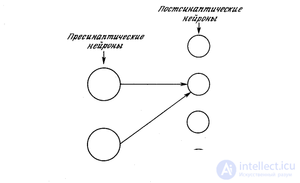
Fig. 10.1. Presynaptic and postsynaptic neurons
In fig. 10.2, it is shown that each neuron is connected only with neurons in the neighboring area, called the communication area. This limitation of the communication region is consistent with the anatomy of the visual cortex, in which neurons rarely interconnect, which are located at a distance of more than one millimeter from each other. In the model under consideration, neurons are ordered in the form of layers with connections from one layer to the next. It is also analogous to the layered structure of the visual cortex and other parts of the brain.
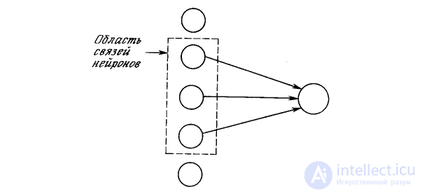
Fig. 10.2. Neuron connections
Since the cognitron is implemented as a multilayered network, complex learning problems arise associated with the selected structure. The author rejected guided learning as being biologically implausible, using teaching without a teacher instead. Obtaining a training set of input images, the network self-organizes by changing the strength of synaptic connections. However, there are no predefined output images that represent the desired network response, but the network is self-tuned to recognize the input images with remarkable accuracy.
The cognitron learning algorithm is conceptually attractive. In the given region of the layer, only the most highly excited neuron is trained. The author compares this with “elite education”, in which only “smart” elements are trained. Those neurons that are already well trained, which is expressed by the power of their arousal, will gain an increment in the power of their synapses in order to further enhance their arousal.
In fig. 10.3 shows that the communication areas of neighboring nodes overlap significantly. This wasteful duplication of functions is justified by mutual competition between the closest nodes. Even if the nodes at the initial moment have absolutely identical output, small deviations always take place; one of the nodes will always have a stronger response to the input image than the neighboring ones. Its strong arousal will have a restraining effect on the excitation of neighboring nodes, and only its synapses will be amplified; neighboring nodes synapses will remain unchanged.
Excitatory neuron. Roughly speaking, the output of the exciting neuron in the cognitron is determined by the ratio of its exciting inputs to the inhibitory inputs. This unusual feature has important advantages, both practical and theoretical.

Fig. 10.3. Area of communication with the area of competition
The total excitatory input to the neuron is the weighted sum of the inputs from the excitatory anterior layer. Similarly, the total input / is the weighted sum of the inputs from all inhibitory neurons. In symbolic form
 ,
,  ,
,
where a i is the weight of the i- th excitatory synapse, u i is the output of the i -th excitatory neuron, b j is the weight of the j- th inhibiting synapse, v j is the output of the j -th inhibitory neuron.
Note that weights have only positive values. The output of the neuron is then calculated as follows:

OUT = NET, with NET≥0,
OUT = 0, with NET <0.
Assuming that the .NET has a positive value, it can be written as follows:

When the inhibitory input is small ( I << 1), OUT can be approximated as
OUT = E - I,
which corresponds to the expression for the usual linear threshold element (with a zero threshold).
The cognitron learning algorithm allows the weights of synapses to grow without restrictions. Due to the absence of a mechanism to reduce weights, they simply increase in the learning process. In conventional linear threshold elements, this would result in an arbitrarily large element output. In the cognitron, the large exciting and decelerating inputs result in a restricting formula of the form:
 if E >> 1 and I >> 1.
In this case, the OUT is determined by the ratio of the drive inputs to the brake inputs, and not by their difference. Thus, the OUT value is limited if both inputs increase in the same X range . Assuming that this is the case, E and I can be expressed as follows:
E = pX , I = qX , p , q - constants,
and after some transformations
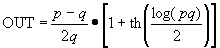 .
.
This function increases according to the Weber-Fechner law, which is often used in neurophysiology to approximate nonlinear input / output ratios of sensory neurons. When using this ratio, the neuron of the cognitron exactly emulates the response of biological neurons. This makes it both a powerful computing element and an accurate model for physiological modeling.
Braking neurons. In the cognitron layer consists of exciting and braking nodes. As shown in fig. 10.4, the neuron of layer 2 has a communication region for which it has synaptic connections with a set of neuron outputs in layer 1. Similarly, in layer 1, there is a inhibitory neuron having the same communication region. The synaptic weights of the inhibitory nodes do not change in the learning process; their weights are predetermined in such a way that the sum of the weights in any of the inhibitory neurons is one. In accordance with these limitations, the output of the inhibiting node INHIB is the weighted sum of its inputs, which in this case represent the arithmetic average of the outputs of the excitatory neurons to which it is connected. In this way,

Fig. 10.4. Cognitron layers
 ,
,
Where  c i is the exciting weight i .
Learning procedure. As explained earlier, the weights of the excitatory neurons change only when the neuron is excited more strongly than any of the nodes in the competition area. If so, the change in the learning process of any of its weights can be defined as follows:
δ a i = qc j u j j ,
where c j is the inhibiting weight of the connection of neuron j in layer 1 with the inhibiting neuron i , and j is the output of neuron j in layer 1, and i is the exciting weight i , q is the normalizing learning factor.
The change in the inhibitory weights of neuron i in layer 2 is proportional to the ratio of the weighted sum of the exciting inputs to the doubled inhibiting input. Calculations are performed by the formula
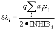 .
.
When there are no excited neurons in the area of competition, other expressions are used to change the weights. This is necessary because the learning process starts with zero weights; therefore, initially there are no excited neurons in any area of competition, and learning cannot be done. In all cases when there is no winner in the field of competition of neurons, the change in the weights of neurons is calculated as follows:
Δ a i = q ' c j u j , δ b i = q ' INHIB,
where q ' is a positive learning factor smaller than q .
This tuning strategy ensures that nodes with a large response force the excitatory synapses that they control to grow larger than the inhibiting synapses. Conversely, nodes that have a low response cause a small increase in excitatory synapses, but a greater increase in inhibitory synapses. Thus, if node 1 in layer 1 has a larger output, the synapse a 1 will increase more than the synapse b 1 . Conversely, the nodes having a small output will provide a small value for the increment a i . However, other nodes in the communication region will be energized, thereby increasing the INHIB signal and b i values.
In the process of learning, the weights of each node in layer 2 are adjusted in such a way that together they constitute a pattern that corresponds to the images that are often presented in the learning process. When a similar image is presented, the template corresponds to it and the node produces a large output signal. A very different image produces a low yield and is usually suppressed by competition.
Lateral braking. In fig. 10.4, each neuron of layer 2 is shown to receive lateral inhibition from neurons located in its competition area. A braking neuron sums up the inputs from all neurons in the area of competition and generates a signal that tends to slow down the target neuron. This method is spectacular, but from a computational point of view it is slow. It covers a large feedback system including every neuron in the layer; to stabilize it may require a large number of computational iterations.
To speed up the calculations in [2], an ingenious method of accelerated lateral braking is used (Fig. 10.5). Here, an additional lateral braking unit processes the output of each excitation unit to simulate the required lateral braking. First, it determines a signal equal to the total inhibitory effect in the area of competition:

Fig. 10.5. Accelerated deceleration
 ,
,
where OUT i is the output of the i - th neuron in the field of competition, g i - the weight of the connection from this neuron to the laterally braking neuron; g i selected in such a way that  .
.
The output of the inhibitory neuron OUT 'is then calculated as follows:
Due to the fact that all the calculations associated with this type of lateral inhibition, are non-recursive, they can be carried out in one pass for the layer, thereby determining the effect in the form of great savings in calculations.
This method of lateral inhibition solves another difficult problem. Suppose that a node in layer 2 is excited strongly, but the excitation of neighboring nodes decreases gradually with increasing distance. When using conventional lateral braking, only the central node will be trained. Other nodes determine that the center node in their area of competition has a higher output. With the proposed lateral braking system, such a situation cannot happen. Many nodes can be trained at the same time and the learning process is more reliable.
Receiving area. The analysis carried out up to this point has been simplified by considering only one-dimensional layers. In reality, the cognitron was designed as a cascade of two-dimensional layers, and in this layer each neuron receives inputs from a set of neurons on the part of the two-dimensional plan that makes up its communication region in the previous layer.
From this point of view, the cognitron is organized like the human visual cortex, which is a three-dimensional structure consisting of several different layers. It turns out that each layer of the brain implements different levels of generalization; the input layer is sensitive to simple images, such as lines, and their orientation in certain areas of the visual area, while the reaction of other layers is more complex, abstract, and independent of the position of the image.
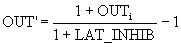
Similar functions are implemented in the cognitron by modeling the organization of the visual cortex. In fig. 10.6, cognitron neurons in layer 2 are shown to react to a specific small area of input layer 1. Neuron in layer 3 is associated with a set of neurons of layer 2, thereby reacting indirectly to a wider set of neurons of layer 1. Similarly, neurons in subsequent layers are more sensitive to wide areas of the input image until each neuron in the output layer responds to the entire input field.
If the connection area of neurons has a constant size in all layers, a large number of layers are required to cover the entire input field with output neurons. The number of layers can be reduced by expanding the bonding area in subsequent layers. Unfortunately, the result of this may be so much overlap of the communication areas that the neurons of the output layer will have the same reaction. To solve this problem can be used to expand the area of competition. Since in this area of competition only one node can be excited, the effect of a small difference in the responses of the neurons of the output layer increases.
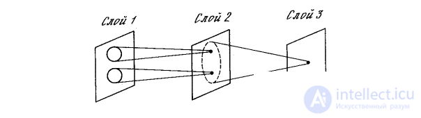
Fig. 10.6. Cognitron Linkages
Alternatively, connections to the previous layer can be distributed probabilistically with most synaptic connections in a limited area and with longer connections that occur much less frequently. This reflects the probabilistic distribution of neurons found in the brain. In a cognitron, this allows each neuron of the output layer to respond to the full input field in the presence of a limited number of layers.
Simulation results The results of computer modeling of a four-layer cognitron, intended for pattern recognition purposes, are described in [4]. Each layer consists of an array of 12x12 excitatory neurons and the same number of inhibitory neurons. The communication area is a square that includes 5x5 neurons. The competition area has a rhombus shape in height and width of five neurons. Lateral inhibition covers the region of 7x7 neurons. The normalizing learning parameters are set in such a way that q = 16.0 and q ' = 2.0. Synapse weights are initialized to 0.
The network was trained by presenting five stimulating images, representing images of Arabic numerals from 0 to 4, on the input layer. The weights of the network were adjusted after the presentation of each digit, the input set was fed to the network input cyclically until each image was presented a total of 20 times.
The effectiveness of the learning process was assessed by running the network in reverse mode; output images, which are the reaction of the network, were fed to the output neurons and propagated back to the input layer. The images obtained in the input layer were then compared with the original input image. To do this, the usual unidirectional connections were assumed to be conducting in the opposite direction and the lateral inhibition was turned off. In fig. 10.7 shows typical test results. Column 2 shows the images produced by each digit on the network output. Эти образы возвращались обратно, вырабатывая на входе сети образ, близкий к точной копии исходного входного образа. Для столбца 4 на выход сети подавался только выход нейрона, имеющего максимальное возбуждение. Результирующие образы в точности те же, что и в случае подачи полного выходного образа, за исключением цифры 0, для которой узел с максимальным выходом располагался на периферии и не покрывал полностью входного поля.

Fig. 10.7. Результаты экспериментов с когнитроном

Comments
To leave a comment
Pattern recognition
Terms: Pattern recognition