Lecture
The convolutional neural network ( pers . Convolutional neural network , CNN ) is a special architecture of artificial neural networks proposed by Jan Lecun and aimed at effective image recognition , is part of the deep learning technology (eng. Deep learning ). Uses some features of the visual cortex , in which the so-called simple cells that react to straight lines from different angles and complex cells, whose reaction is associated with the activation of a certain set of simple cells, were discovered. Thus, the idea of convolutional neural networks is the alternation of convolutional layers (eng. Convolution layers ) and sub-sampling layers (eng. subsampling layers , subsample layers). The network structure is unidirectional (without feedback), essentially multi-layered. Standard methods are used for teaching, most often the method of back propagation of error. The activation function of neurons (transfer function) - any, at the choice of the researcher.
The network architecture got its name because of the convolution operation, the essence of which is that each image fragment is multiplied by the convolution matrix (core) element by element, and the result is summed up and written to the similar position of the output image.
The machine learning convolutional neural network (SNA, Eng. Convolutional neural network, CNN, ConvNet) - is a type of artificial neural network feedforward in which individual neurons are enclosed so that they react in the area of the visual field , which partly overlap. The convolution of the network was inspired by biological processes, they are variations of multilayer perceptrons designed to use minimal pre-processing. they are widely used in image and video recognition, recommender systems and natural language processing.
Convolutional neural networks (SNS). It sounds like a strange combination of biology and mathematics with an admixture of computer science, but no matter how it sounds, these networks are one of the most influential innovations in the field of computer vision. For the first time, neural networks attracted universal attention in 2012, when Alex Krizhevski won the ImageNet contest (roughly speaking, this is an annual computer vision competition), lowering the record of classification errors from 26% to 15%, which was a breakthrough. Today, in-depth learning is at the core of many companies' services: Facebook uses neural networks for automatic tagging, Google for searching user photos, Amazon for generating product recommendations, Pinterest for personalizing the user's home page, and Instagram for the search infrastructure.
When used for image recognition, convolutional neural networks (SNS) consist of several layers of small collections of neurons that process portions of the input image called receptive fields. The outputs of these collections are then stacked so that they overlap, to get a better representation of the primary image, this is repeated for each such layer. The overlap conclusion allows the SNC to be tolerant of parallel translations of the input image.
Convolutional networks can include layers of a local or global subsample that combine the outputs of clusters of neurons. They also consist of various combinations of zgortkovih and fully connected layers, using pointwise nonlinearity at the end of each layer. to reduce the number of free parameters and improve the generalization, a convolution operation on small input areas is introduced. One of the main advantages of zgortkovyh networks is the use of joint weight in zgortkovyh layers, which means that the same filter (weight bank) is used for each pixel of the layer; it both reduces the amount of required memory and improves performance.
Very similar zgortkovih neural network architecture is also used and some neural network with a time delay , particularly intended for the recognition tasks and / or classification of images as to enter into neuron outputs may be performed at regular intervals, a convenient way to analyze the images.
Compared to other image classification algorithms, convolutional neural networks use relatively little pre-processing. This means that the network is responsible for learning the filters; in traditional algorithms, they were developed manually. The lack of dependence in the development of attributes from a priori knowledge and human effort is a great advantage of the NRO.
The development of convolutional neural networks followed the discovery of visual mechanisms in living organisms. Early work in 1968 showed that the visual cortex animal contains a complex arrangement of cells that are sensitive to light in the identification of small sub-areas of the visual field, which overlap, these receptive fields. This work has identified two main types of cells: simple cells , reacting the most special konturopodibni images in their receptive fields, and complex cells , which have large receptive fields, and is locally invariant to the exact position of the image. These cells act as local filters over the input space.
Neocognitron, the predecessor of convolutional networks, was presented in a 1980 paper. In 1988, their number was developed separately, with explicit parallel and learning-capable convolutions for signals propagating in time. Their design was improved in 1998, generalized 2003 and the same year simplified. The famous LeNet-5 network can successfully classify numbers, and is used to recognize numbers in checks. However, with more complex tasks, the breadth and depth of the network increase, and become limited computing resources and hamper performance.
In 1988, an excellent OHP design was proposed for the decomposition of one-dimensional electromyography signals. 1989, it was modified for other convolution-based schemes.
With the advent of efficient computing on GP, it became possible to train large networks. In 2006, several publications described effective ways to train zgortkovye neural networks with a large number of layers. 2011, they were refined and implemented at the GP, with impressive results. 2012 Chireshan et al. Significantly improved the best performance in the literature for several image sets, including MNIST databases , NORB database, HWDB1.0 character set (Chinese characters), CIFAR10 data set (set of 60000 labeled RGB images 32 × 32) and the ImageNet dataset.
While traditional models of multilayer perceptron successfully applied to image recognition, because of full connectivity between nodes, they suffer from the curse of dimensionality , and therefore does not scale well to the image of the higher resolution.

SNA layers located in 3 dimensions
For example, in the CIFAR-10 set, images are only 32 × 32 × 3 in size (width 32, height 32, 3 color channels), therefore one fully connected neuron in the first hidden layer of an ordinary neural network would be 32 * 32 * 3 = 3072 weights. However, an image of 200 × 200 will result in neurons having 200 * 200 * 3 = 120,000 weights.
Such network architectures do not take into account the spatial data structure, considering the input pixels, far and close to each other, on equal terms. It is obvious that the complete connectivity of neurons in the framework of image recognition is wasteful, and a huge number of parameters quickly lead to retraining.
Convolutional neural networks are biologically inspired variants of multilayer perceptrons designed to mimic the behavior of the visual cortex. These models mitigate the challenges posed by the BSB architecture, using the strong spatially local correlation present in natural images. In contrast to the BSH, CNN has the following distinguishing features:
Together, these properties allow zgortkovye neural networks to achieve a better generalization on the tasks of vision. Weight sharing also helps, dramatically reducing the number of free parameters that need to be learned, thus reducing memory requirements for the network. Reducing the amount of memory allows training large, powerful networks.
The CNN architecture is formed by a stack of different layers that transform the input volume into an output volume (which, for example, saves the level of relation to classes) using a differentiated function. Typically, several different types of layers are used. We will discuss them below:
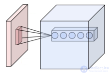
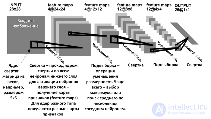
In a conventional perceptron, which is a fully connected neural network, each neuron is connected to all the neurons of the previous layer, and each connection has its own personal weighting factor. In the convolutional neural network, only a limited matrix of small weights is used in the convolution operation, which is “moved” across the entire layer being processed (at the very beginning, directly in the input image), forming after each shift an activation signal for the neuron of the next layer with a similar position. That is, for different neurons of the output layer, the total weights are used - the weights matrix, which is also called the weights set or the convolution core.. It is constructed in such a way that it graphically encodes a single sign, for example, the presence of an inclined line at a certain angle. Then the next layer, resulting from the convolution operation with such a matrix of weights, shows the presence of this inclined line in the layer being processed and its coordinates, forming the so-called feature map (English feature map).). Naturally, in the convolutional neural network a set of scales is not one, but a whole gamma encoding various lines and arcs from different angles. Moreover, such convolution kernels are not laid by the researcher in advance, but are formed independently by training the network using the classical error propagation method. Passing with each set of scales forms its own copy of the feature map, making the neural network multidimensional (many independent feature maps on one layer). It should also be noted that when a layer is weighed by a matrix of weights, it is usually moved not by a full step (the size of this matrix), but by a small distance. So, for example, if the dimension of the 5 × 5 weights matrix is, it is shifted by one or two neurons (pixels) instead of five, in order not to “step over” the desired feature.
Operation subsampling (Engl. Subsampling , Engl. Pooling , also translated as "subsampling operation" or union operation), performs the dimensionality reduction formed signs cards. In this network architecture, it is considered that information on the presence of the desired feature is more important than accurate knowledge of its coordinates, therefore the maximum is selected from several neighboring neurons of the feature map and is taken as one reduced-dimension neuron. Also sometimes used the operation of finding the average between neighboring neurons. Due to this operation, in addition to speeding up further calculations, the network becomes more invariant to the scale of the input image.
Thus, repeating one after another several layers of convolution and subsampling, a convolutional neural network is constructed. The alternation of layers allows mapping of features from feature maps, which in practice means the ability to recognize complex feature hierarchies. Usually, after passing through several layers, a map of signs degenerates into a vector or even a scalar, but there are hundreds of such maps of signs. At the output of the network, it is often additionally installed several layers of a fully connected neural network (perceptron), to the input of which end character maps are fed.
If on the first layer the convolution core passes through only one source image, then on the inner layers the same core runs parallel to all feature maps of this layer, and the result of the convolution is summed up , forming (after passing the activation function) the trait map of the next layer corresponding to this convolution kernel.
The convolutional network model, which we consider in this article, consists of three types of layers: convolutional layers, subsampling (subsampling, subsample) layers and layers of the “ordinary” neural network - the perceptron .
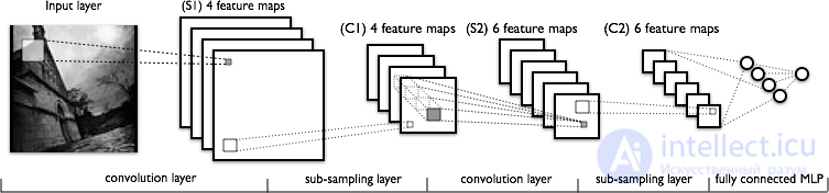
Fig.1: a convolutional network diagram (from http://deeplearning.net)
The first two types of layers (convolutional, subsampling), alternating with each other, form the input feature vector for a multilayer perceptron. The network can be trained using gradient methods .
The name of the convolution network was named after the operation, the convolution , it is often used for image processing and can be described by the following formula.

Here f is the original image matrix, g is the convolution core (matrix).
Informally, this operation can be described as follows: we pass the window of kernel size g with a given step (usually 1) the entire image f, at each step we elementwise multiply the window contents by the kernel g, the result is summed up and written into the result matrix.
However, depending on the processing method of the edges of the original matrix, the result may be less than the original image (valid), the same size (same) or larger (full).
|
|
|
|
In this section we will look at the device of the convolutional layer.
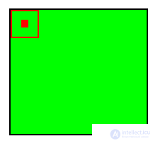
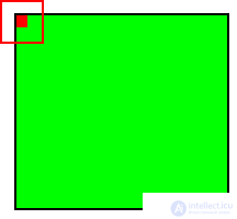
The convolutional layer implements the idea of the so-called. local receptive fields, i.e. Each output neuron is connected only to a certain (small) area of the input matrix and thus models some features of human vision.
In simplified form, this layer can be described by the following formula.

Here x l is the output of the layer l, f () is the activation function, b is the shift coefficient, the ∗ symbol denotes the convolution of the input x with the kernel k.
In this case, due to the edge effects, the size of the original matrices is reduced.
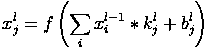
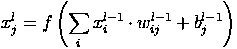
Here x j l is the feature map j (layer output l), f () is the activation function, b j is the shift coefficient for feature map j, k j is the convolution kernel number j, x i l − 1 are the feature maps of the previous layer.
In this section we’ll talk about subsampling layer. Layers of this type perform a reduction in the size of the input feature map (usually 2 times). This can be done in different ways, in this case we will consider the method of selecting the maximum element (max-pooling) - the entire attribute map is divided into 2x2 element cells, from which the maximum values are selected. Formally, the layer can be described as follows.

Here x l is the output of the layer l, f () is the activation function, a, b are the coefficients, subsample () is the operation of sampling local maximum values.
Using this layer allows you to improve the recognition of samples with a modified scale (reduced or enlarged).
The last of the types of layers is the layer of the “ordinary” multilayer perceptron (MLP), it can be described by the following relation.
Here x l is the output of the layer l, f () is the activation function, b is the shear coefficient, w is the matrix of weight coefficients.
In this section we will talk about the scheme of the connection of the layers to each other.
Consider a convolutional network of 7 layers, their order is described below.
At the same time, neurons (feature maps) of the second downsampling layer and the third convolutional layer are connected selectively, i.e. in accordance with the adjacency matrix, which is specified as a network parameter. For a network with the number of attribute cards in the second layer 7 and 9 in the third layer, it may look like this.
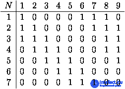
Table 1: Example of Convolutional Layer Connectivity Matrix
Thus, each output card is formed by a partial sum of the results of convolutions of the input cards, for each such partial amount its own set of convolution kernels.
Connecting all the cards of the second layer with all the cards of the third layer would significantly increase the number of connections.
Connecting one-to-one maps would be another repetition of convolution that was already present between the layers.
As a rule, the network architect himself decides on what principle to organize the connection of layer maps.
The zgortkovih layer (English Convolutional layer ) is the main building block of OHP. Layer parameters consist of a set of filters for learning (or cores), which have a small receptive field, but extend to the entire depth of the input volume. During the straight pass, each filter performs convolution along the width and height of the input volume, calculating the product of the filter and input data, and forming a 2-dimensional map of the activation of this filter. As a result, the network learns which filters are activated when they see a particular specific type of feature in a certain spatial position at the entrance.
The compilation of activation maps of all filters along the depth measurement forms the total initial volume of the convolutional layer. Thus, each entry in the source volume can also be interpreted as the output of a neuron, which looks at a small area in the input, and shares the parameters with the neurons of the same activation card.
Local connectivity
When processing high-dimensional inputs such as images, it is impractical to connect neurons with all neurons of the previous volume, since this network architecture does not take into account the spatial structure of the data. Convolutional networks use a spatially local correlation by providing a localized circuit between the neurons of adjacent layers: each neuron connects to only a small area of the incoming volume. The entire volume of this food is a hyperparameter , which is called the receptive field of the neuron. Connections are local in space (along the width and height), but always propagate along the entire depth of the incoming volume. This architecture ensures that trained filters produce a strong response to spatially local input images.
Spatial organization
The size of the output volume of the convolutional layer is controlled by three hyper parameters : depth , pitch and zero complement .
The spatial size of the output volume can be calculated as a function of the size of the input volume
продолжение следует...
Часть 1 Convolutional neural network (convolutional neural network -CNN)

Comments
To leave a comment
Pattern recognition
Terms: Pattern recognition