Analysis of existing approaches to face recognition

Despite the large variety of algorithms presented, one can identify the general structure of the facial recognition process:


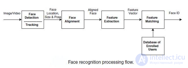The overall processing of facial image recognition

At the first stage, the face is detected and localized in the image. At the recognition stage, the image of the face is aligned (geometric and luminance), the calculation of the signs and the recognition itself is the comparison of the calculated signs with the standards embedded in the database. The main difference of all the algorithms presented will be the calculation of signs and the comparison of their aggregates among themselves.

1. The method of flexible comparison on graphs (Elastic graph matching) [13].

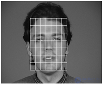
The essence of the method is reduced to the elastic juxtaposition of graphs describing images of faces. Persons are represented as graphs with weighted vertices and edges. At the recognition stage, one of the graphs - the reference one - remains unchanged, while the other is deformed in order to best fit the first one. In such recognition systems, graphs can be either a rectangular grid or a structure formed by characteristic (anthropometric) points of a face.

but)

b)

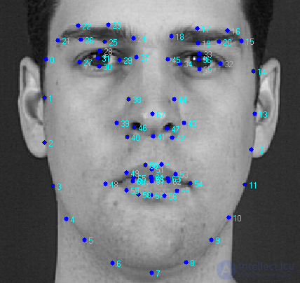
An example of the structure of a graph for face recognition: a) a regular lattice b) a graph based on anthropometric points of the face.

At the vertices of the graph, the values ​​of attributes are computed, most often using the complex values ​​of Gabor filters or their ordered sets — Gabor wavelets (Gabor lines), which are computed locally in some local vertex region of the graph by convolving the pixel brightness values ​​with Gabor filters.


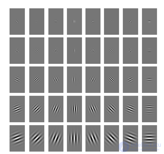Set (bank, jet) filters Gabor


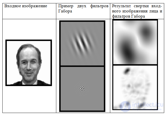An example of a convolution image of the face with two Gabor filters

The edges of the graph are weighted by the distances between adjacent vertices. The difference (distance, discriminatory characteristic) between two graphs is calculated with the help of some price deformation function, which takes into account both the difference between the values ​​of features calculated at the vertices and the degree of deformation of the edges of the graph.
A graph is deformed by displacing each of its vertices by a certain distance in certain directions relative to its original location and selecting its position such that the difference between the values ​​of attributes (responses of Gabor filters) at the top of the deformed graph and the corresponding top of the reference graph is minimal. This operation is performed alternately for all vertices of the graph until the smallest total difference between the signs of a deformable and reference graphs is reached. The value of the price function of the strain in such a position of the deformable graph will be a measure of the difference between the input image of the face and the reference graph. This “relaxation” deformation procedure should be performed for all reference persons included in the system database. The system recognition result is the standard with the best value of the price function of deformation.


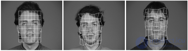An example of the deformation of a graph in the form of a regular lattice

In individual publications, 95-97% recognition efficiency is indicated, even in the presence of various emotional expressions and a change in the face angle of up to 15 degrees. However, developers of elastic comparison systems on graphs refer to the high computational cost of this approach. For example, to compare an input face image with 87 reference ones, it took approximately 25 seconds when working on a parallel computer with 23 transputers [15] (Note: the publication is dated 1993). In other publications on this topic, time is either not indicated, or it is said that it is great.

Disadvantages: high computational complexity of the recognition procedure. Low manufacturability in memorizing new standards. Linear dependence of work time on the size of the database of persons.

2. Neural networks

Currently, there are about a dozen varieties of neural networks (NA). One of the most widely used options is a network built on a multilayer perceptron, which allows you to classify the image / signal fed to the input according to the network pre-tuning / training.
Neural networks are trained on a set of training examples. The essence of learning is reduced to adjusting the weights of interneuronal connections in the process of solving an optimization problem using the gradient descent method. In the process of learning the NA, the key features are automatically extracted, their importance is determined, and the relationships between them are built. It is assumed that a trained NA will be able to apply the experience gained in the learning process to unknown images at the expense of generalizing abilities.
The best results in the field of face recognition (based on the analysis of publications) were shown by the Convolutional Neural Network or the convolutional neural network (hereinafter referred to as SNS) [29-31], which is a logical development of the ideas of NA architectures like cognitron and neocognitron. Success is due to the possibility of taking into account the two-dimensional topology of the image, in contrast to the multilayer perceptron.
Distinctive features of the SNA are local receptor fields (provide local two-dimensional connectivity of neurons), total weights (provide detection of some features anywhere in the image) and a hierarchical organization with spatial subsampling. Thanks to these innovations, the SNA provides partial stability to scale changes, shifts, turns, angle changes and other distortions.


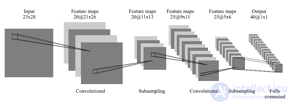Schematic representation of the convolutional neural network architecture

Testing the SNA on an ORL database containing images of individuals with small changes in lighting, scale, spatial turns, position, and various emotions showed 96% recognition accuracy.
The development of the SNA received in the development of DeepFace [47], which acquired
Facebook to recognize the faces of users of your social network. All features of the architecture are closed.


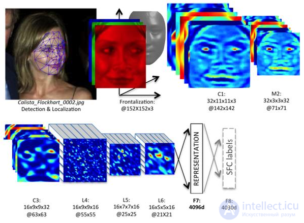DeepFace working principle

Disadvantages of neural networks: adding a new reference person to the database requires a complete retraining of the network throughout the entire set (quite a long procedure, depending on the sample size from 1 hour to several days). Mathematical problems associated with learning: hitting the local optimum, choosing the optimal optimization step, retraining, etc. The step of choosing a network architecture (number of neurons, layers, nature of connections) is difficult to formalize. Summarizing all the above, we can conclude that NA is a “black box” with difficult to interpret work results.

3. Hidden Markov models (SMM, HMM)

One of the statistical methods of face recognition are hidden Markov models (SMM) with discrete time [32-34]. The SMMs use the statistical properties of the signals and take into account their spatial characteristics directly. The elements of the model are: the set of hidden states, the set of observable states, the transition probability matrix, the initial probability of states. Each has its own Markov model. When an object is recognized, Markov models generated for a given object base are checked and the maximum observable probability is searched for that the sequence of observations for a given object is generated by the corresponding model.
To date, it has not been possible to find examples of the commercial use of SMM for face recognition.

Disadvantages:
- it is necessary to select the model parameters for each database;
- The SMM does not have a distinctive ability, that is, the learning algorithm only maximizes the response of each image to its model, but does not minimize the response to other models.

4. Principal component method or principal component analysis (PCA) [11]

One of the most well-known and developed is the principal component analysis (PCA) method, based on the Karhunen-Loyev transform.
Initially, the principal component method began to be used in statistics to reduce the feature space without significant loss of information. In the problem of face recognition, it is mainly used to represent a face image with a small dimension vector (main components), which is then compared with the reference vectors embedded in the database.
The main goal of the principal component method is to significantly reduce the dimension of the feature space in such a way that it describes as best as possible the “typical” images belonging to many individuals. Using this method, it is possible to identify various variability in a training sample of facial images and describe this variability in the basis of several orthogonal vectors, which are called eigenface (eigenface).

The set of eigenvectors obtained once on a training sample of face images is used to encode all other face images, which are represented by a weighted combination of these eigenvectors. Using a limited number of eigenvectors, it is possible to obtain a compressed approximation to the input face image, which can then be stored in a database as a coefficient vector, which simultaneously serves as a search key in a database of persons.

The essence of the main component method is as follows. First, the entire training set of faces is transformed into one common data matrix, where each row is a single copy of the image of a person laid out in a row. All persons of the training set must be reduced to the same size and with normalized histograms.


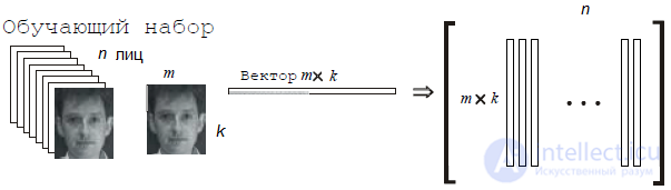Transformation of the training set of persons into one common matrix X

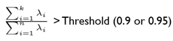
Then the data is normalized and the rows are brought to the 0th average and 1st dispersion, the covariance matrix is ​​calculated. For the resulting covariance matrix, the problem of determining the eigenvalues ​​and the corresponding eigenvectors (proper faces) is solved. Next, the eigenvectors are sorted in descending order of eigenvalues ​​and only the first k vectors are left by the rule:



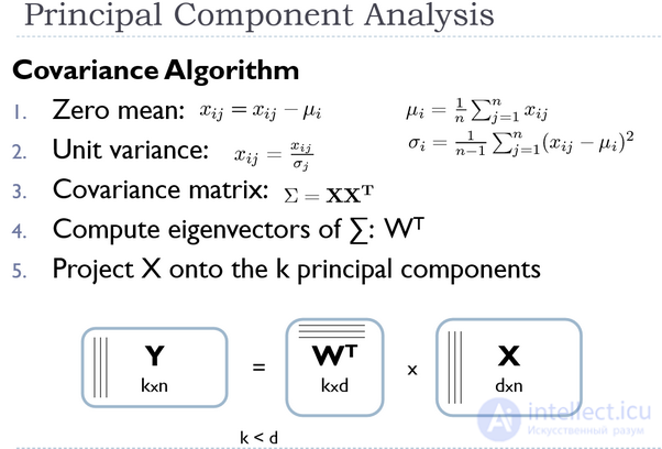PCA algorithm


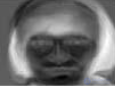
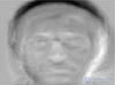
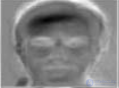
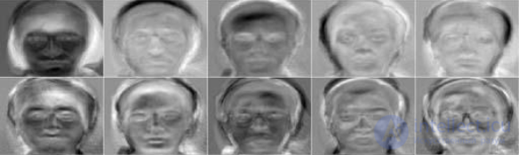An example of the first ten eigenvectors (own faces) obtained on the learner set of faces

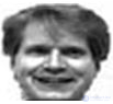
= 0.956 * -1.842 * +0.046 ...

An example of the construction (synthesis) of a human face using a combination of its own faces and main components


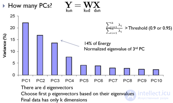The principle of choosing the basis of the first best eigenvectors


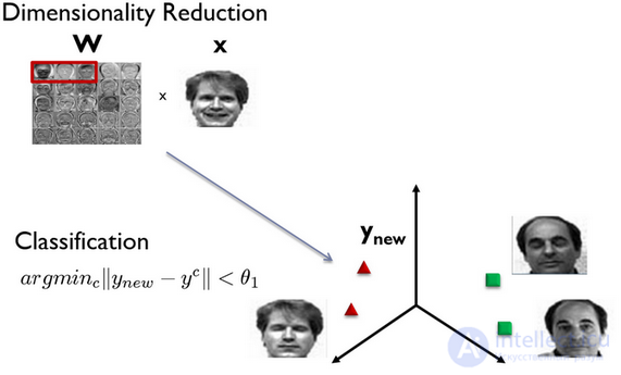An example of mapping a face into a three-dimensional metric space, obtained from three own faces and further recognition



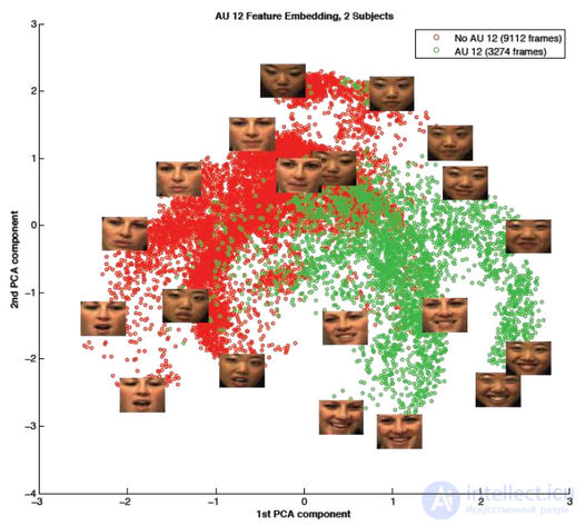
The principal component method has proven itself in practical applications. However, in cases where there are significant changes in the light or facial expression on the face, the effectiveness of the method drops significantly. The thing is, the PCA chooses a subspace so as to approximate the input data set as much as possible, rather than discriminate between classes of individuals.

[22] proposed a solution to this problem with the use of the linear discriminant Fisher (in the literature the name “Eigen-Fisher”, “Fisherface”, LDA) is found. LDA selects a linear subspace that maximizes the relationship:



Where

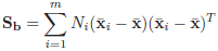
interclass scatter matrix, and


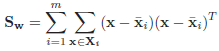
Matrix of intraclass scatter; m is the number of classes in the database.

LDA is looking for a projection of data in which classes are as linearly separable as possible (see figure below). For comparison, the PCA is looking for a data projection in which the spread across the entire database of individuals will be maximized (excluding classes). According to the results of experiments [22], under conditions of strong tank and lower shading of face images, Fisherface showed 95% efficiency compared to 53% of the Eigenface.


The fundamental difference in the formation of PCA and LDA projections

PCA versus LDA

5. Active Appearance Models (AAM) and Active Shape Models (ASM) (Habra Source)

Active Appearance Models (AAM)
Active Models of Appearance (Active Appearance Models, AAM) are statistical models of images that can be adapted to a real image by various kinds of deformations. This type of model in a two-dimensional version was proposed by Tim Kuts and Chris Taylor in 1998 [17,18]. Initially, active appearance models were used to evaluate the parameters of facial images.
The active appearance model contains two types of parameters: parameters associated with the form (form parameters) and parameters associated with the statistical model of image pixels or texture (appearance parameters). Before using the model should be trained on a set of pre-marked images. Image marking is done manually. Each label has its own number and determines the characteristic point that the model will have to find when adapting to a new image.


An example of a markup of a face image of 68 points forming the AAM shape

The AAM learning procedure begins with the normalization of the shapes on the tagged images in order to compensate for differences in scale, tilt and offset. For this, the so-called generalized Procrustes analysis is used.


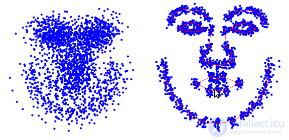Coordinates of face shape points before and after normalization

Of the total set of normalized points, the main components are then selected using the PCA method.


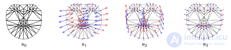The AAM form model consists of a s0 triangulation lattice and a linear combination of si offsets with respect to s0

Further, a matrix is ​​formed from pixels inside the triangles formed by points of the shape, such that each column contains the pixel values ​​of the corresponding texture. It is worth noting that the textures used for learning can be either single-channel (grayscale) or multi-channel (for example, RGB color space or another). In the case of multichannel textures, the vectors of pixels are formed separately for each of the channels, and then they are concatenated. After finding the main components of the texture matrix, the AAM model is considered trained.



The AAM appearance model consists of a base view A0, defined by pixels inside the base lattice s0 and a linear combination of offsets Ai relative to A0



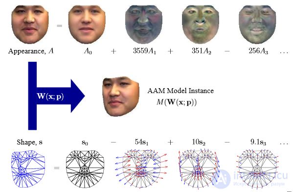
An example of instantiation AAM. Form Parameters Vector
p = (p_1, p_2, 〖..., p _m) ^ T = (- 54.10, -9.1, ...) ^ T is used to synthesize the model of the form s, and the vector of parameters λ = (λ_1, λ_2, 〖..., λ〗 _m) ^ T = (3559,351, -256, ...) ^ T for the synthesis of the appearance of the model. The resulting face model 〖M (W (x; p))〗 ^ is obtained as a combination of two models — shape and appearance.

The model is fitted to a specific face image in the process of solving an optimization problem, the essence of which is to minimize the functionality



gradient descent method. The parameters of the model found in this way will reflect the position of the model on a specific image.



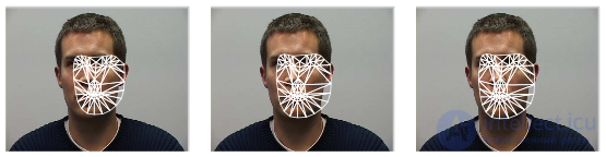
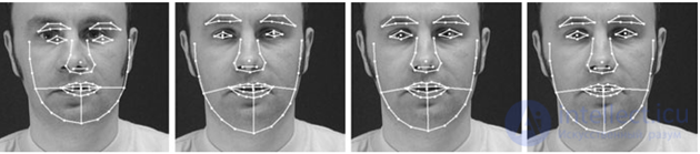
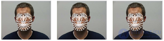An example of fitting a model to a specific image in 20 iterations of the gradient descent procedure.

With AAM, you can model images of objects subject to both hard and non-rigid deformation. AAM consists of a set of parameters, some of which represent the shape of the face, the rest define its texture. The deformation is usually understood as a geometric transformation in the form of a composition of translation, rotation and scaling.When solving the problem of localizing a face in an image, a search is made for parameters (location, shape, texture) of AAM, which represent the synthesized image that is closest to the observed one. According to the proximity of AAM to the customized image, a decision is made whether there is a face or not.

Active Shape Models (ASM)

The essence of the ASM method [16,19,20] is to take into account the statistical relationships between the location of anthropometric points. On the available sample of images of persons taken in full face. On the image, the expert marks the location of the anthropometric points. Each image points are numbered in the same order.



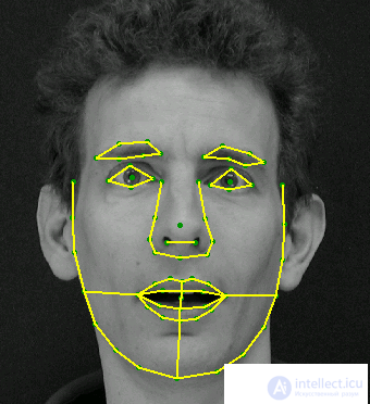
Example of a face shape using 68 points

In order to bring the coordinates on all the images to a single system, usually so-called is performed. generalized scrolling analysis, as a result of which all points are reduced to the same scale and centered. Next, for the whole set of patterns, the average form and the covariance matrix are calculated. On the basis of the covariance matrix, eigenvectors are calculated, which are then sorted in descending order of the corresponding eigenvalues. The ASM model is defined by the matrix Φ and the vector of the average form s ̅.
Then any form can be described with the help of the model and parameters:



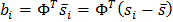
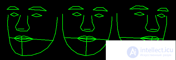
The localization of the ASM model on a new, not included in the training sample image is carried out in the process of solving the optimization problem.


a B C D)
Illustration ASM model localization process on a specific image: a) an initial position b) after 5 iterations) after 10 iterations g) the model has converged

, however, still the main purpose of AAM and ASM is not a face detection and precise location of the face and anthropometric points on the image for further processing.

In almost all algorithms, a mandatory step that precedes the classification is the alignment, which refers to the alignment of the face image to the frontal position relative to the camera or to bring a set of persons (for example, in a training set for classifier training) to a single coordinate system. To implement this stage, it is necessary to localize the image of anthropometric points characteristic of all persons — most often these are the centers of the pupils or the corners of the eyes. Different researchers distinguish different groups of such points. In order to reduce computational costs for real-time systems, developers allocate no more than 10 such points [1].

The AAM and ASM models are designed to precisely localize these anthropometric points in the image of the face.

6. The main problems associated with the development of facial recognition systems

Illumination



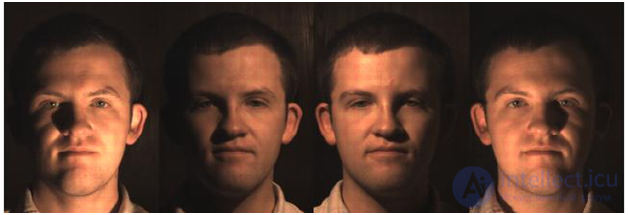
problem The problem of the position of the head (the face is, nevertheless, a 3D object).



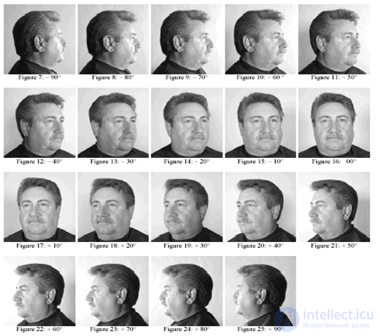
In order to assess the effectiveness of the proposed face recognition algorithms, the DARPA agency and the research laboratory of the US Army have developed a face recognition technology (FERET) program.

Algorithms based on flexible comparison on graphs and various modifications of the principal component method (PCA) took part in the large-scale tests of the FERET program. The efficiency of all algorithms was about the same. In this regard, it is difficult or even impossible to distinguish clearly between them (especially if the test dates are agreed). For frontal images taken on the same day, the acceptable recognition accuracy is usually 95%. For images made by different devices and with different lighting, accuracy, as a rule, drops to 80%. For images made with a difference of a year, the recognition accuracy was about 50%. It is worth noting that even 50 percent is more than acceptable accuracy of the system of this kind.

Each year, FERET publishes a report on the comparative testing of modern facial recognition systems [55] on the basis of more than one million. Unfortunately, the latest reports do not disclose the principles of building recognition systems, but only the results of the work of commercial systems are published. To date, the leading is the NeoFace system developed by NEC.