It is not easy to keep track of all the neural network architectures that continually arise lately. Even understanding all the abbreviations that professionals throw at first may seem like an impossible task.
Therefore, I decided to make a cheat sheet for such architectures. Most of them are neural networks, but some are animals of a different breed. Although all these architectures are presented as new and unique, when I portrayed their structure, internal communications have become much clearer.
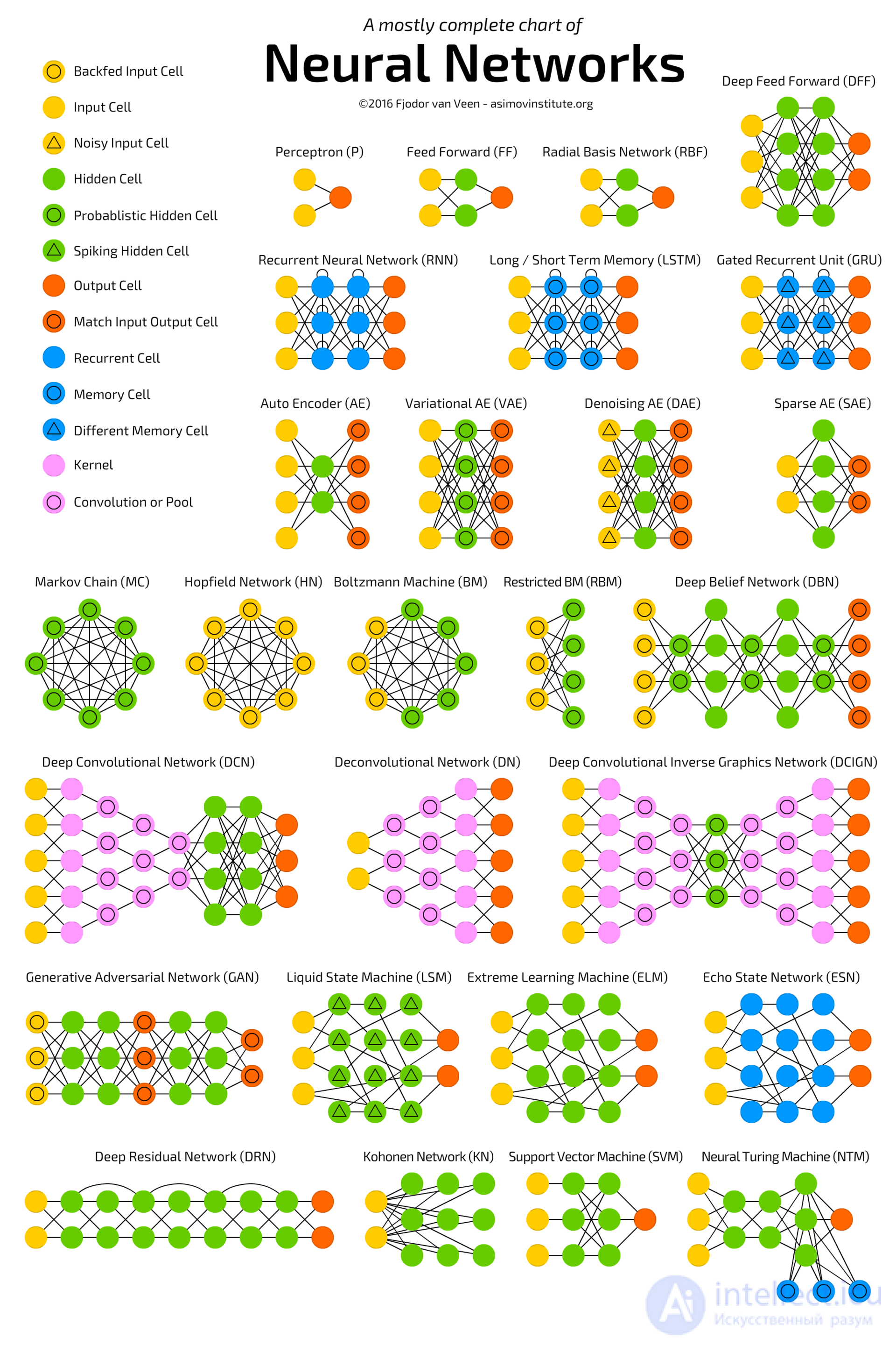
The image of neural networks in the form of graphs has one drawback: the graph will not show how the network works. For example, a variational autoencoder (variational autoencoders, VAE) looks exactly like a simple autoencoder (AE), while the learning process of these neural networks is completely different. Usage scenarios differ even more: in VAE, noise comes in from the input from which they receive a new vector, while AE simply finds the closest corresponding vector to the input data from those that they “remember”. I will also add that this review has no purpose to explain the work of each of the topologies from the inside (but this will be the topic of one of the following articles).
It should be noted that not all (although most) of the abbreviations used here are generally accepted. RNN is sometimes understood as recursive neural networks, but usually this abbreviation means recurrent neural network. But that's not all: in many sources you will find RNN as a designation for any recurrent architecture, including LSTM, GRU, and even bidirectional options. Sometimes a similar confusion occurs with AE: VAE, DAE and the like can simply be called AE. Many abbreviations contain different amounts of N at the end: you can say “convolutional neural network” - CNN (Convolutional Neural Network), or you can just “convolutional network” - CN.
It is almost impossible to compile a complete list of topologies, since new ones appear constantly. Even if you specifically look for publications, it can be difficult to find them, and some can simply be overlooked. Therefore, although this list will help you create an idea of the world of artificial intelligence, please do not consider it exhaustive, especially if you read the article long after its appearance.
For each of the architectures shown in the diagram, I gave a very short description. Some of them will be useful if you are familiar with several architectures, but are not specifically familiar with this one.
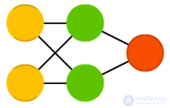
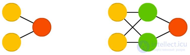 Direct-distribution networks (Feed forward neural networks, FF or FFNN) and perceptrons (Perceptrons, P) are
 very simple — they transfer information from input to output. It is believed that neural networks have layers, each of which consists of input, hidden or output neurons. Neurons of one layer are not connected with each other, with each neuron of this layer associated with each neuron of the adjacent layer. The simplest working network consists of two input and one output neuron and can simulate a logic gate - the basic element of a digital circuit that performs an elementary logic operation. FFNN is usually trained in the back-propagation method of error, feeding models to the input of a pair of input and expected output data. The error is usually understood to mean different degrees of deviation of the output from the original (for example, the standard deviation or the sum of the absolute values of the differences). Provided that the network has a sufficient number of hidden neurons, in theory it will always be able to establish a connection between the input and output data. In practice, the use of direct distribution networks is limited, and more often they are shared with other networks.
Rosenblatt, Frank. “The perceptron: a probabilistic model for information storage in the brain.” Psychological review 65.6 (1958): 386.
Original Paper PDF
 Radial basis functions (RBF)
 networks are FFNN with a radial basis function as an activation function. There is nothing more to add. We do not want to say that it is not used, but the majority of FFNN with other activation functions usually are not separated into separate groups.
Broomhead, David S., and David Lowe. Radial basis functions, multi-variable functional interpolation and adaptive networks. No. RSRE-MEMO-4148. ROYAL SIGNALS AND RADAR ESTABLISHMENT MALVERN (UNITED KINGDOM), 1988.
Original Paper PDF
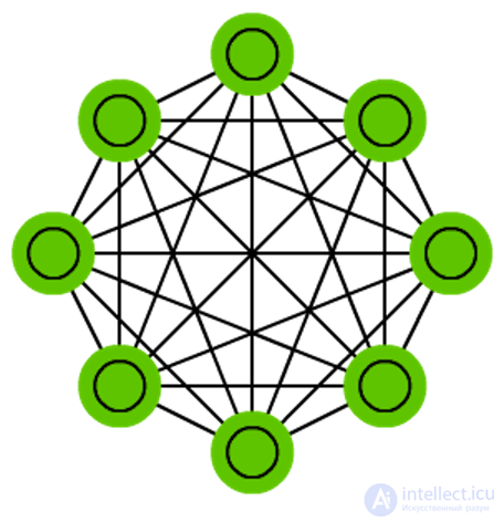
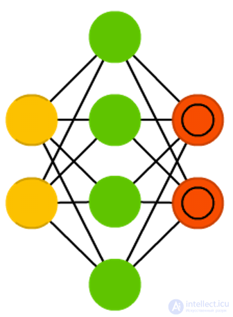
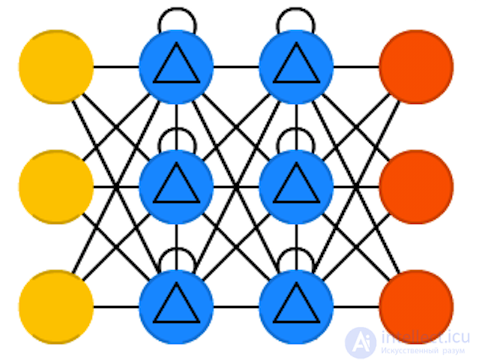
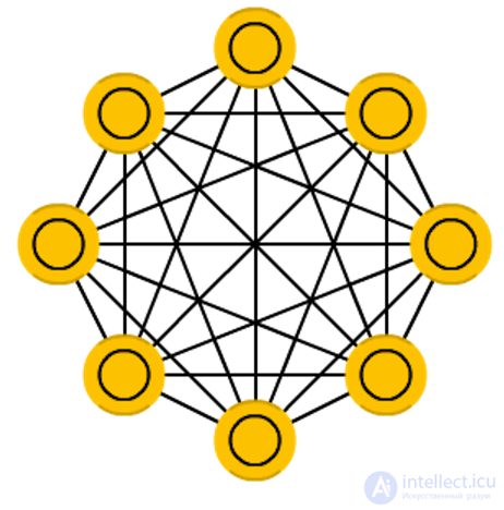 The Hopfield neural network
 is a fully connected network (each neuron is connected to each), where each neuron appears in all three forms. Each neuron serves as an input to learning, hidden during it and a weekend after. The weights matrix is selected in such a way that all the “memorized” vectors are proper for it. Once a system is trained in one or more images, it will converge to one of its known images, because only one of these states is stationary. Note that this does not necessarily correspond to the desired state (unfortunately, we do not have a magic black box). The system is only partially stabilized due to the fact that the total “energy” or “temperature” of the network gradually decreases during training. Each neuron has an activation threshold commensurate with this temperature, and if the sum of the input data exceeds this threshold, the neuron can go into one of two states (usually -1 or 1, sometimes 0 or 1). Network nodes can be updated in parallel, but most often it happens sequentially. In the latter case, a random sequence is generated, which determines the order in which the neurons will update their state. When each of the neurons is updated and their state no longer changes, the network comes to a stationary state. Such networks are often called associative memory, since they converge with the state closest to the given one: as a person, seeing half of the picture, can finish drawing the missing half, so does the neural network, getting a half-noisy picture at the entrance, completes it to the whole.
Hopfield, John J. “Emergency collective computational abilities and systems”. ”79.8 (1982): 2554-2558.
Original Paper PDF
 Markov Chains (Markov Chains, MC or discrete time Markov Chain, DTMC)
 are a kind of predecessor of Boltzmann machines (BM) and Hopfield networks (HN). In Markov chains, we set the transition probabilities from the current state to the neighboring ones. In addition, this chain has no memory: the subsequent state depends only on the current one and does not depend on all past states. Although the Markov chain cannot be called a neural network, it is close to them and forms the theoretical basis for BM and HN. Markov chains are also not always fully connected.
Hayes, Brian. “First links in the Markov chain.” American Scientist 101.2 (2013): 252.
Original Paper PDF
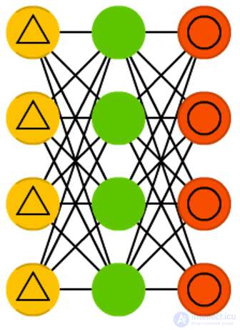
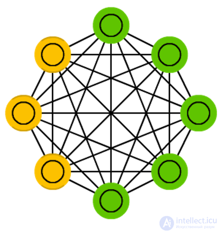 Boltzmann machines (BM) machines are
 in many ways similar to the Hopfield network, but in them some neurons are marked as input and some remain hidden. Input neurons become output when all neurons in the network update their states. First, weights are assigned randomly, then backward propagation occurs, or more recently, using the contrastive divergence algorithm (when the gradient is calculated using a Markov chain). BM is a stochastic neural network, since the Markov chain is involved in the training. The process of learning and working here is almost the same as in the Hopfield network: certain initial states are assigned to neurons, and then the chain begins to function freely. In the process of work, neurons can assume any state, and we constantly move between input and hidden neurons. Activation is governed by the value of the total temperature, with a decrease in which the energy of the neurons is reduced. Reducing energy causes stabilization of neurons. Thus, if the temperature is set correctly, the system reaches an equilibrium.
Hinton, Geoffrey E., and Terrence J. Sejnowski. “Learning and releasing in Boltzmann machines.” Parallel distributed processing: Exploration in the microstructure of cognition 1 (1986): 282-317.
Original Paper PDF
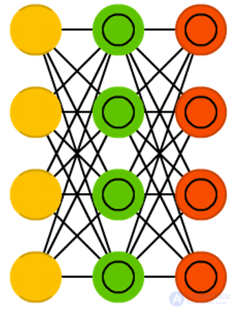
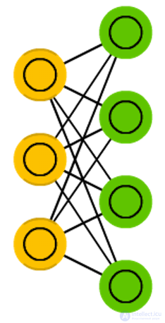 The limited Boltzmann machine (Restricted Boltzmann machine, RBM) is
 , surprisingly, very similar to the normal Boltzmann machine. The main difference between RBM and BM is that they are limited and therefore more convenient to use. In them, each neuron is not connected with each, but only each group of neurons is connected to other groups. Input neurons are not connected to each other, there are no connections and between hidden neurons. RBM can be trained in the same way as FFPN, with a small difference: instead of transferring data forward and subsequent back propagation of error, data is transmitted back and forth (to the first layer), and then forward and backward propagation is applied .
Smolensky, Paul. Information processing in dynamical systems: Foundations of harmony theory. No. CU-CS-321-86. COLORADO UNIV AT BOULDER DEPT OF COMPUTER SCIENCE, 1986.
Original Paper PDF
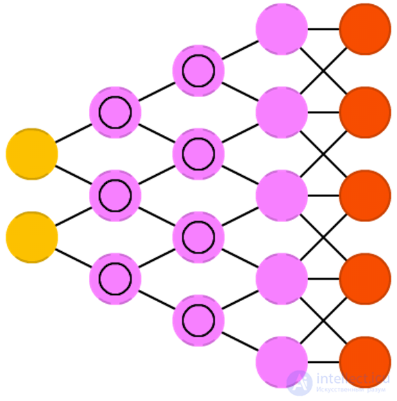
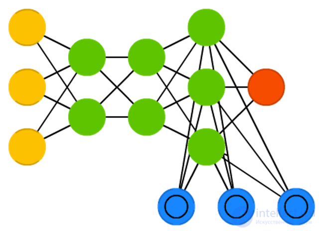
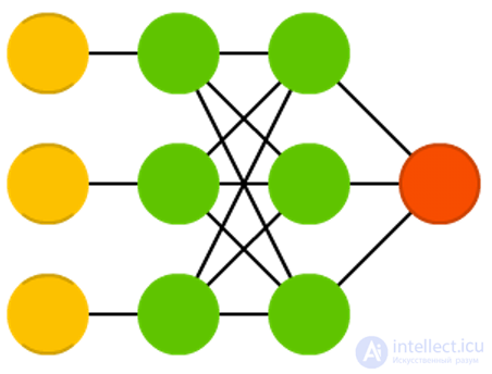
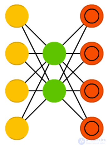 Autoencoders (AE)
 - something like FFNN, this is rather a different way to use FFNN than a fundamentally new architecture. The main idea of avtoenkoderov - automatic encoding (as when compressing, and not when encrypting) information, hence the name. The network resembles an hourglass shape, since the hidden layer is smaller than the input and output; moreover, it is symmetric with respect to the middle layers (one or two, depending on the parity / oddness of the total number of layers). The smallest layer is almost always the middle one, information is maximally compressed in it. All that is located to the middle - the coding part, above the middle - decoding, and in the middle (you will not believe) - the code. AE is trained in the back propagation method of an error, giving input data and setting an error equal to the difference between the input and the output. AE can be constructed symmetric and in terms of weights, exposing the encoding weights equal decoding.
Bourlard, Hervé, and Yves Kamp. “Auto-association by multilayer perceptrons and singular value decomposition.” Biological cybernetics 59.4-5 (1988): 291-294.
Original Paper PDF
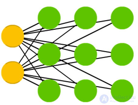
 A sparse autoencoder (Sparse autoencoder, AE)
 is to some extent the opposite of AE. Instead of teaching the network to represent blocks of information in a smaller “space,” we encode information so that it takes up more space. And instead of forcing the system to converge in the center, and then expand back to its original size, we, on the contrary, increase the middle layers. Networks of this type can be used to extract many small details from a data set. If we started teaching SAE in the same way as AE, we would get in most cases an absolutely useless network, where the output is exactly the same as at the input. To avoid this, instead of the input data, we output the input data plus a penalty for the number of activated neurons in the hidden layer. To a certain extent, this resembles a biological neural network (spiking neural network), in which not all neurons are constantly in an excited state.
Marc'Aurelio Ranzato, Christopher Poultney, Sumit Chopra, and Yann LeCun. “Efficient learning of an energy-based model.” Proceedings of NIPS. 2007
Original Paper PDF
The architecture of
variational autoencoders (VAE) is the same as that of ordinary, but they are taught another - the approximate probability distribution of input samples. This is to some extent a return to basics, as the VAE is a little closer to the Boltzmann machines. However, they rely on Bayesian mathematics regarding probabilistic judgments and independence, which are intuitive, but require complex calculations. The basic principle can be formulated as follows: take into account the degree of influence of one event on another. If a certain event occurs in one place, and another event happens somewhere else, then these events are not necessarily related. If they are not related, then the propagation of the error should take this into account. This is a useful approach, since neural networks are a kind of huge graphs, and sometimes it is useful to exclude the influence of some neurons on others, falling into the lower layers.
Kingma, Diederik P., and Max Welling. “Auto-encoding variational bayes.” ArXiv preprint arXiv: 1312.6114 (2013).
Original Paper PDF
 Noise-canceling (noise-resistant) auto-encoders (Denoising autoencoders, DAE)
 - this is AE, which we do not just input data to the input, but noise data (for example, making the image more grainy). Nevertheless, we calculate the error by the former method, comparing the output sample with the original without noise. Thus, the network does not memorize small details, but large features, since memorizing small details that are constantly changing due to noise often leads nowhere.
Vincent, Pascal, et al. “Extracting and composing robust features with denoising autoencoders.” 25th international conference on Machine Learning. ACM, 2008.
Original Paper PDF
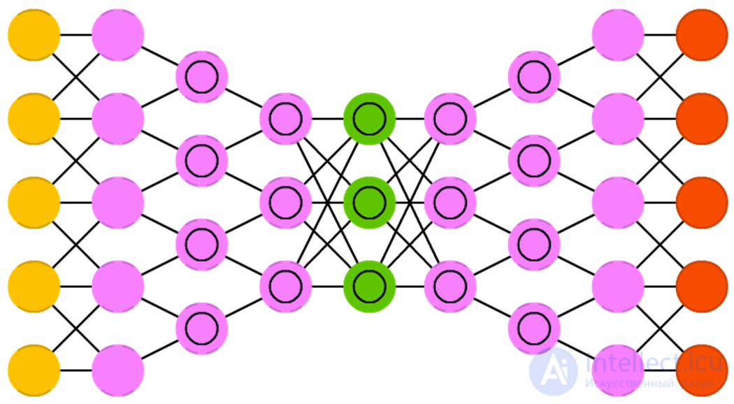
 Deep trust networks (Deep belief networks, DBN)
 are networks composed of several RBM or VAE. Such networks proved to be effectively trained one after another, when each network must learn to code the previous one. This method is also called “greedy learning”, it is to make the best decision at the moment to get a suitable, but perhaps not the optimal result. DBNs can be trained by contrastive divergence or backpropagation and learn to present data as a probabilistic model, exactly like RBM or VAE. Once a trained and stationary model can be used to generate new data.
Bengio, Yoshua, et al. “Greedy layer-wise training of deep networks.” Advances in neural information processing systems 19 (2007): 153.
Original Paper PDF
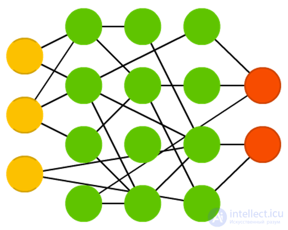
 Convolutional neural networks (convolutional neural networks, CNN) and deep convolutional neural networks (deep convolutional neural networks, DCNN) are
 radically different from other networks. They are mainly used for image processing, sometimes for audio and other types of input data. A typical way of using CNN is image classification: if a cat image is input, the network will issue a cat, if the dog's picture is a dog. Such networks typically use a “scanner” that does not process all data at one time. For example, if you have an image of 200x200, you want to build a network layer of 40 thousand nodes. Instead, the network counts a 20x20 square (usually from the upper left corner), then moves 1 pixel and counts a new square, and so on. Notice that we do not break the image into squares, but rather we crawl on it. These inputs are then transmitted through convolutional layers, in which not all nodes are interconnected. Instead, each node is connected only to its nearest neighbors. These layers tend to shrink with depth, and usually they are reduced by one of the dividers of the amount of input data (for example, 20 nodes in the next layer will turn into 10, in the next - in 5), often used degrees of two. In addition to convolutional layers, there are also so-called pooling layers. Association is a way to reduce the dimension of the data received, for example, the most red pixel is selected and transmitted from a 2x2 square. In practice, by the end of CNN attach FFNN for further data processing. Such networks are called deep (DCNN), but their names are usually interchangeable.
LeCun, Yann, et al. “Gradient-based learning to document recognition.” Proceedings of the IEEE 86.11 (1998): 2278-2324.
Original Paper PDF
Deployed neural networks (deconvolutional networks, DN) , also called reverse graphical networks, are conversely neural networks. Imagine that you transmit the word “cat” to the network and train it to generate pictures of cats by comparing the resulting pictures with real images of cats. DNN can also be combined with FFNN. It should be noted that in most cases the network does not transmit a string, but a binary classifying vector: for example, <0, 1> is a cat, <1, 0> is a dog, and <1, 1> is both a cat and a dog. Instead of combining layers, which are often found in CNN, there are similar inverse operations, usually interpolation or extrapolation.
Zeiler, Matthew D., et al. “Deconvolutional networks.” Computer Vision and Pattern Recognition (CVPR), 2010 IEEE Conference on. IEEE, 2010.
Original Paper PDF
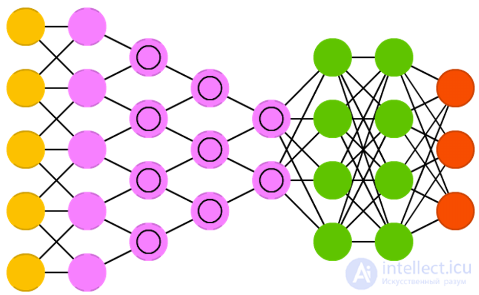
The name “Deep convolutional inverse graphics networks (DCIGN)" can be misleading, because in reality these are variational autoencoders with convolutional and sweeping networks as encoding and decoding parts, respectively. Such networks present the features of the image as probabilities and can learn to build an image of a cat and a dog together, looking only at the pictures with cats and only dogs. In addition, you can show this network a photo of your cat with an annoying neighbor with and ask her to cut out the dog and the images, and DCIGN will cope with this task, even if it has never done anything like that. The developers also demonstrated that DCIGN can simulate various complex image transformations, such as changing the light source or turning 3D objects. teach back propagation.
Kulkarni, Tejas D., et al. “Deep convolutional inverse graphics network.” Advances in Neural Information Processing Systems. 2015
Original Paper PDF
Генеративные состязательные сети (Generative adversarial networks, GAN) принадлежат другому семейству нейросетей, это близнецы — две сети, работающие вместе. GAN состоит из любых двух сетей (но чаще это сети прямого распространения или сверточные), где одна из сетей генерирует данные (“генератор”), а вторая — анализирует (“дискриминатор”). Дискриминатор получает на вход или обучающие данные, или сгенерированные первой сетью. То, насколько точно дискриминатор сможет определить источник данных, служит потом для оценки ошибок генератора. Таким образом, происходит своего рода соревнование, где дискриминатор учится лучше отличать реальные данные от сгенерированных, а генератор стремится стать менее предсказуемым для дискриминатора. Это работает отчасти потому, что даже сложные изображения с большим количеством шума в конце концов становятся предсказуемыми, но сгенерированные данные, мало отличающиеся от реальных, сложнее научиться отличать. GAN достаточно сложно обучить, так как задача здесь — не просто обучить две сети, но и соблюдать необходимый баланс между ними. Если одна из частей (генератор или дискриминатор) станет намного лучше другой, то GAN никогда не будет сходиться.
Goodfellow, Ian, et al. “Generative adversarial nets.” Advances in Neural Information Processing Systems. 2014.
Original Paper PDF

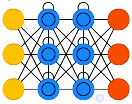
Рекуррентные нейронные сети (Recurrent neural networks, RNN) — это те же сети прямого распространения, но со смещением во времени: нейроны получают информацию не только от предыдущего слоя, но и от самих себя в результате предыдущего прохода. Следовательно, здесь важен порядок, в котором мы подаем информацию и обучаем сеть: мы получим разные результаты, если сначала скормим ей “молоко”, а затем “печеньки”, или если сначала “печеньки”, а потом уже “молоко”. У RNN есть одна большая проблема — это проблема исчезающего (или взрывного) градиента: в зависимости от используемой функции активации информация со временем теряется, так же как и в очень глубоких сетях прямого распространения. Казалось бы, это не такая уж серьезная проблема, так как это касается только весов, а не состояний нейронов, но именно в весах хранится информация о прошлом; если вес достигнет значения 0 или 1 000 000, то информация о прошлом состоянии станет не слишком информативной. RNN могут использоваться в самых разнообразных областях, так как даже данные, не связанные с течением времени (не звук или видео) могут быть представлены в виде последовательности. Картинка или строка текста могут подаваться на вход по одному пикселю или символу, так что вес будет использоваться для предыдущего элемента последовательности, а не для того, что случилось X секунд назад. В общем случае, рекуррентные сети хороши для продолжения или дополнения информации, например, автодополнения.
Elman, Jeffrey L. “Finding structure in time.” Cognitive science 14.2 (1990): 179-211.
Original Paper PDF
Долгая краткосрочная память (Long short term memory, LSTM) — попытка побороть проблему взрывного градиента, используя фильтры (gates) и блоки памяти (memory cells). Эта идея пришла, скорее, из области схемотехники, а не биологии. У каждого нейрона есть три фильтра: входной фильтр (input gate), выходной фильтр (output gate) и фильтр забывания (forget gate). Задача этих фильтров — сохранять информацию, останавливая и возобновляя ее поток. Входной фильтр определяет количество информации с предыдущего шага, которое будет храниться в блоке памяти. Выходной фильтр занят тем, что определяет, сколько информации о текущем состоянии узла получит следующий слой. Наличие фильтра забывания на первый взгляд кажется странным, но иногда забывать оказывается полезно: если нейросеть запоминает книгу, в начале новой главы может быть необходимо забыть некоторых героев из предыдущей. Показано, что LSTM могут обучаться действительно сложным последовательностям, например, подражать Шекспиру или сочинять простую музыку. Стоит отметить, что так как каждый фильтр хранит свой вес относительно предыдущего нейрона, такие сети достаточно ресурсоемки.
Hochreiter, Sepp, and Jürgen Schmidhuber. “Long short-term memory.” Neural computation 9.8 (1997): 1735-1780.
Original Paper PDF
Управляемые рекуррентные нейроны (Gated recurrent units, GRU) — разновидность LSTM. У них на один фильтр меньше, и они немного иначе соединены: вместо входного, выходного фильтров и фильтра забывания здесь используется фильтр обновления (update gate). Этот фильтр определяет и сколько информации сохранить от последнего состояния, и сколько информации получить от предыдущего слоя. Фильтр сброса состояния (reset gate) работает почти так же, как фильтр забывания, но расположен немного иначе. На следующие слои отправляется полная информация о состоянии — выходного фильтра здесь нет. В большинстве случаем GRU работают так же, как LSTM, самое значимое отличие в том, что GRU немного быстрее и проще в эксплуатации (однако обладает немного меньшими выразительными возможностями).
Chung, Junyoung, et al. “Empirical evaluation of gated recurrent neural networks on sequence modeling.” arXiv preprint arXiv:1412.3555 (2014).
Original Paper PDF
Нейронные машины Тьюринга (Neural Turing machines, NMT) можно определить как абстракцию над LSTM и попытку “достать” нейросети из “черного ящика”, давая нам представление о том, что происходит внутри. Блок памяти здесь не встроен в нейрон, а отделен от него. Это позволяет объединить производительность и неизменность обычного цифрового хранилища данных с производительностью и выразительными возможностями нейронной сети. Идея заключается в использовании адресуемой по содержимому памяти и нейросети, которая может читать из этой памяти и писать в нее. Они называются нейронными машинами Тьюринга, так как являются полными по Тьюриингу: возможность читать, писать и изменять состояние на основании прочитанного позволяет выполнять все, что умеет выполнять универсальная машина Тьюринга.
Graves, Alex, Greg Wayne, and Ivo Danihelka. “Neural turing machines.” arXiv preprint arXiv:1410.5401 (2014).
Original Paper PDF
Двунаправленные RNN, LSTM и GRU (BiRNN, BiLSTM и BiGRU) не изображены на схеме, так как выглядят в точности так же, как их однонаправленные коллеги. Разница лишь в том, что эти нейросети связаны не только с прошлым, но и с будущим. Например, однонаправленная LSTM может научиться прогнозировать слово “рыба”, получая на вход буквы по одной. Двунаправленная LSTM будет получать также и следующую букву во время обратного прохода, открывая таким образом доступ к будущей информации. А значит, нейросеть можно обучить не только дополнять информацию, но и заполнять пробелы, так, вместо расширения рисунка по краям, она может дорисовывать недостающие фрагменты в середине.
Schuster, Mike, and Kuldip K. Paliwal. “Bidirectional recurrent neural networks.” IEEE Transactions on Signal Processing 45.11 (1997): 2673-2681.
Original Paper PDF
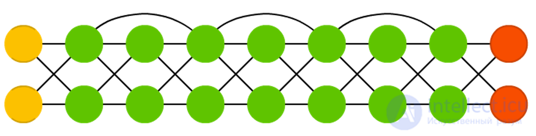
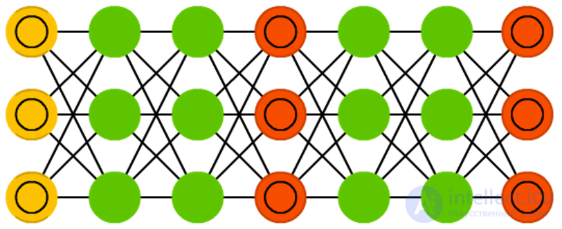
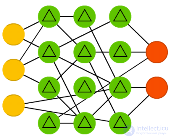
Deep residual networks (Deep Resualual Networks, DRN) are very deep FFNNs with additional connections between layers, usually two to five, connecting not only adjacent layers, but also more distant ones. Instead of looking for a way to find the input data corresponding to the source data through, say, five layers, the network is trained to assign an “output block + input block” pair to the input block. Thus, the input data passes through all layers of the neural network and is served on a platter to the last layers. It was shown that such networks can be trained in patterns with a depth of up to 150 layers, which is much more than can be expected from an ordinary 2-5-layer neural network. However, it has been proven that networks of this type are actually just RNN without explicit use of time, and they are often compared with LSTM without filters.
He, Kaiming, et al. “Deep residual learning for image recognition.” ArXiv preprint arXiv: 1512.03385 (2015).
Original Paper PDF
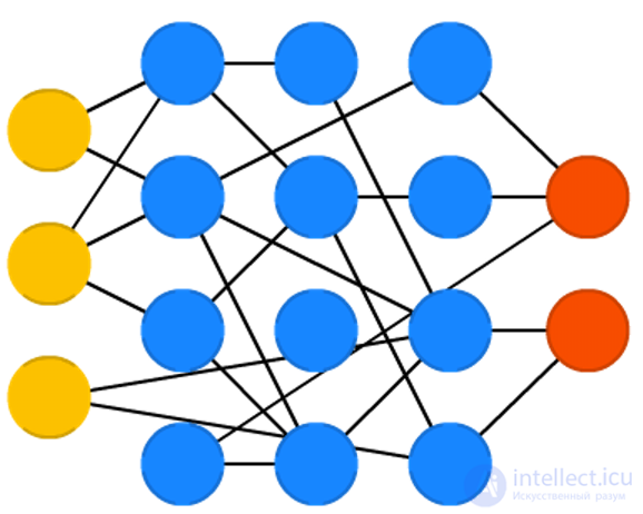
Neural echo networks (Echo state networks, ESN) are another type of recurrent neural networks. They stand out because the connections between the neurons in them are random, not organized into neat layers, and they are trained differently. Instead of submitting data to the input and backward propagation of an error, we transmit data, update the states of the neurons and monitor the output for some time. The input and output layers play a nonstandard role, since the input layer serves to initialize the system, and the output layer - as an observer of the order of activation of neurons, which manifests itself with time. During training, only the connections between the observer and the hidden layers change.
Jaeger, Herbert, and Harald Haas. “Harnessing nonlinearity: Predicting chaotic systems and energy saving in wireless communication.” Science 304.5667 (2004): 78-80.
Original Paper PDF
Extreme learning machines (ELM) are the same FFNN, but with random connections between neurons. They are very similar to LSM and ESN, but are used rather like forward-propagation networks, and this is not due to the fact that they are not recurrent or impulsive, but to the fact that they are trained in the back propagation method.
Cambria, Erik, et al. “Extreme learning machines [trends & controversies].” IEEE Intelligent Systems 28.6 (2013): 30-59.
Original Paper PDF
Liquid state machines (LSM) are similar to ESNs. Their main difference is that LSM is a kind of impulse neural networks: threshold functions come to replace the sigmoidal curve, and each neuron is also a cumulative memory block. When the state of the neuron is updated, the value is not calculated as the sum of its neighbors, but is added to itself. As soon as the threshold is exceeded, the energy is released and the neuron sends an impulse to other neurons.
Maass, Wolfgang, Thomas Natschläger, and Henry Markram. “A new framework for neural computation based on perturbations.” Neural computation 14.11 (2002): 2531-2560.
Original Paper PDF
The support vector machine (SVM) method is used to find optimal solutions in classification problems. In the classical sense, the method is capable of categorizing linearly shared data: for example, determine which figure shows Garfield, and which figure shows Snoopy. In the process of learning, the network places all Garfield and Snoopy on 2D graphics and tries to divide the data with a straight line so that each side has data of only one class and the distance from the data to the line is maximum. Using a trick with the kernel, you can classify data of dimension n. Having built a 3D graph, we can distinguish Garfield from Snoopy and Simon the cat, and the higher the dimension, the more cartoon characters you can classify. This method is not always considered as a neural network.
Cortes, Corinna, and Vladimir Vapnik. “Support-vector networks.” Machine learning 20.3 (1995): 273-297.
Original Paper PDF
Finally, the last inhabitant of our zoo is the Kohonen networks, KN, or organizing (feature) map, SOM, SOFM map of Kohonen. KN uses competitive training to classify data without a teacher. The network analyzes its neurons for maximum match with the input data. The most suitable neurons are updated so as to even closer look like the input data, in addition, the weights of their neighbors are approaching the input data. How much the state of the neighbors changes depends on the distance to the most suitable node. KN is also not always referred to as neural networks.
Kohonen, Teuvo. “Self-organized formation of topologically correct feature maps.” Biological cybernetics 43.1 (1982): 59-69.
Original Paper PDF

Comments
To leave a comment
Computational Neuroscience (Theory of Neuroscience) Theory and Applications of Artificial Neural Networks
Terms: Computational Neuroscience (Theory of Neuroscience) Theory and Applications of Artificial Neural Networks