Lecture
Probabilistic generalizations of the Hopfield model and the Boltzmann statistical machine. Bidirectional associative memory Kosko. Presentation of information on the Hopfield network that solves the problem of combinatorial optimization. Neurocomputation and neuromathematics. Principles of the organization of computational processes in neuroEVM.
The limitations of the capacity of synaptic memory, as well as the problem of the false memory of a classical neural network in the Hopfield model trained according to Hebb's rule, led to the appearance of a number of studies aimed at removing these limitations. In this case, the main emphasis was placed on modifying the rules of learning.
At the previous lecture it was established that the orthogonality of the images of the training sample is a very favorable circumstance, since in this case it is possible to show their stable preservation in memory. In the case of exact orthogonality, the maximum memory capacity is reached, equal to N - the maximum possible number of orthogonal images from the N components.
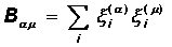
One of the most frequently used ways to improve Hebb's rule is based on this property of orthogonal images: the initial images should be orthogonalized before memorizing in the neural network. the orthogonalization procedure leads to a new kind of memory matrix:

where B -1 is the matrix inverse to matrix B:
This form of the memory matrix ensures the reproduction of any set of p <N images. However, a significant disadvantage of this method is its nonlocality : learning to communicate between two neurons requires knowledge of the states of all other neurons. In addition, before you start learning, you need to know in advance all the training images. Adding a new image requires a complete re-training of the network. Therefore, this approach is very far from the original biological bases of the Hopfield-Hebb network, although in practice it leads to noticeable improvements in its functioning.
Another approach to improving the Hebbian rule is to eliminate synaptic connection symmetry. The memory matrix can be selected in the following form:
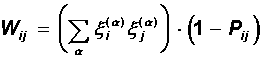
The elements of the matrix P ij from the set {0,1} control the presence or absence of a connection from neuron i to neuron j.
An increase in the memory capacity in such a model can in principle be achieved due to the appearance of new degrees of freedom associated with the matrix P. In the general case, however, it is difficult to suggest an algorithm for choosing this matrix. It should also be noted that a dynamic system with an asymmetric matrix does not need to be stable.
The possibility of forgetting unnecessary, unnecessary information is one of the remarkable properties of biological memory. The idea of applying this property to the Hopfield artificial neural network is “surprisingly” simple: when memorizing images of a training set, false images are also remembered with them. They should be “forgotten”.
The corresponding algorithms are called unmasking algorithms. The essence of them is as follows.
In the first phase, the network is trained according to the standard Hebb's rule. Memory is filled with true images and a lot of false information. At the next phase (the uncoupling phase) of the network, a certain (random) image l (0) is presented. The network evolves from the state l (0) to a certain state l (f) , which with a large volume of the training sample most often turns out to be false. Now the matrix of relations can be corrected in order to reduce the depth of the minimum energy corresponding to this false state:
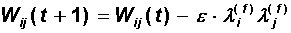
As a degree of forgetting e , a small number is chosen, which guarantees a slight deterioration of useful memory, if the state l (f) does not turn out to be false. After several “forgetting sessions,” network properties improve (JJHopfield et al, 1983).
This procedure is far from a formal theoretical substantiation, but in practice it leads to a more regular energy surface of the neural network and to an increase in the volume of pools of attraction of useful images.
The further development of neural network architectures of associative memory was obtained in the works of Bart Kosko (B. Kosko, 1987). He proposed a model of heteroassociative memory in which associations between pairs of images are remembered. Memorization takes place in such a way that when a network of one of the images is displayed, the second member of the pair is restored.
Memorization of images through the associations between them is very characteristic of human memory. The recollection (reproduction) of the necessary information can occur by building a chain of associations. For example, watching the smoke from the factory pipe on the street, you may well remember that you left the kettle on the stove at home.
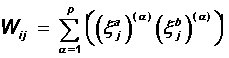
The bi-directional network in Kosko’s model consists of two layers of neurons (layer A and layer B). The connections between the layers are arranged in such a way that each neuron of one layer is connected with each neuron of another layer. There are no connections between neurons inside the layers, the number of neurons on each layer may be different. Pairs of images ( x a , x b ) ( a ) , a = 1..p are intended for memorization. Training is governed by the Hebba rule:
The dynamics of the system is parallel and occurs according to the formulas:
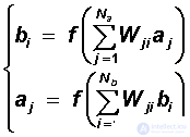
Here {a j }, j = 1..N a is the activity states of the neurons of the layer A, {b i }, i = 1..N b - layer B. The threshold function or sigmoid can be used as the neural function f. In the particular case of identical layers and identical images in training pairs, the Kosko network is completely equivalent to the Hopfield model.
During the iterative dynamics of the state of the neurons of layer A, they cause changes in the states of the neurons of layer B, which, in turn, modify the states of neurons A, and so on. Iterations, as well as in the Hopfield network, converge, because the matrix of relations is symmetric. When a network is shown, only an image on layer A will also restore the corresponding image on layer B, and vice versa.
The Kosko network also has the property of auto-association: if some fragments of images on layer A and B are known at the same time, then in the process of dynamics both images of the pair will be simultaneously restored.
In the previous lecture, the classical Hopfield model with binary neurons was considered. The change in the states of neurons in time was described by deterministic rules, which at a given point in time unambiguously determined the degree of excitation of all neurons of the network.
The evolution in the state space of the Hopfield network is completed at a stationary point — the local minimum of energy. In this state, any changes in the activity of any neuron are prohibited, since they lead to an increase in the energy of the network. If we continue to draw an analogy between classical neurodynamics and statistical (dynamic) systems in physics, then we can introduce the concept of temperature of a statistical ensemble of neurons. The behavior of the Hopfield network corresponds to the zero temperature (full freezing) of the statistical system.
At a strictly zero temperature (T = 0), the statistical Boltzmann factor ~ exp (- D E / T) makes it impossible to increase the energy. The transition to non-zero temperatures (T> 0) significantly enriches the dynamics of the system, which now with a non-zero probability of making transitions with increasing E and visiting new statistical states.
Let's return to neural networks. For some neurons, the possibility of transition to a state with greater energy means a refusal to follow a deterministic law of state change. At nonzero temperatures, the state of the neuron is determined in a probabilistic way:
S i (t + 1) = sign (h i (t) - Q ), with probability P i
S i (t + 1) = - sign (h i (t) - Q ), with probability (1-P i )
The probability of transition to a state with increasing energy is the smaller, the greater the difference in the energies of the final E 2 and initial E 1 states. In statistical systems, this probability is determined by the Boltzmann formula:
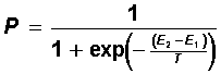
It is easy to see that, in the low-temperature limit (T ® 0), the probability P tends to unity, and the dynamics transform into ordinary deterministic neurodynamics.
At high temperatures (T >> D E) the probability is P = 1/2, i.e. A change in the state of a neuron is in no way connected either with its previous state or with the value of the “neural field” h (t). Network states change completely randomly, and the situation does not resemble a system with memory.
The dynamics of the neural system at non-zero temperatures is no longer Lyapunovskaya, since the network energy is no longer obliged to decrease with time. In this case, generally speaking, the network does not fully stabilize - the state will continue to experience changes in which D E µ T.
If the network temperature is now gradually reduced, a large increase in energy becomes less and less likely, and the system freezes in the vicinity of the minimum. It is very important to note that freezing will most likely occur in the bowl of the deepest and widest minimum, i.e. the network mostly reaches a global minimum of energy.
The process of slow cooling and localization of the state in the low-energy region is similar to the process of annealing of metals used in industry for their hardening; therefore, it is called imitation annealing .
Introducing a non-zero temperature into the dynamics of a neural network improves memory properties, since the system ceases to “feel” small local minima corresponding to false images. However, for this you have to pay inaccuracies when reproducing images due to the lack of full stabilization of the system at the minimum point.
The associativity of the memory of the Hopfield neural network is not its only advantage, which is used in practice. Another important feature of this architecture is the reduction of its Lyapunov function in the process of neurodynamics. Consequently, the Hopfield neural network can be considered as an algorithm for optimizing the objective function in the form of network energy.
The class of objective functions that can be minimized by a neural network is quite wide: all bilinear and quadratic forms with symmetric matrices fall into it. On the other hand, a very wide range of mathematical problems can be formulated in the language of optimization problems. This includes such traditional tasks as differential equations in a variational formulation; problems of linear algebra and a system of nonlinear algebraic equations, where a solution is sought in the form of a residual minimization, and others.
Research on the possibility of using neural networks to solve such problems today has created a new scientific discipline - neuromathematics .
The use of neural networks for solving traditional mathematical problems looks very attractive, so neuroprocessors are systems with an extremely high level of parallelism in information processing. In our book, we will consider the use of neuro-optimizers for several other tasks, namely, combinatorial optimization problems.
Many problems of optimal placement and resource planning, route selection, CAD tasks and others, with external seeming simplicity of formulation, have solutions that can be obtained only by exhaustive search of options. Often, the number of options increases rapidly with the number of structural elements N in the problem (for example, as N! - factorial N), and the search for the exact solution for practically useful values of N becomes obviously unacceptably expensive. Such tasks are called non-polynomially complex or NP-complete . If it is possible to formulate such a problem in terms of optimization of the Lyapunov function, then the neural network provides a very powerful tool for finding an approximate solution.
Consider the classic example of an NP-complete problem — the so-called task of the comivarius (roving merchant). There are N cities on the plane, defined by pairs of their geographical coordinates: (x i , y i ), i = 1..N. Someone must, starting with an arbitrary city, visit all these cities, with each going exactly once. The problem is to choose a travel route with the minimum possible total path length.
The total number of possible routes is  , and the task of finding the shortest of them by the brute force method is very laborious. An acceptable approximate solution can be found using a neural network, for which, as already mentioned, it is necessary to reformulate the problem in the language of Lyapunov function optimization (JJHopfield, DWTank, 1985).
Denote the names of cities in capital letters (A, B, C, D ...). An arbitrary route can be presented in the form of a table in which the unit in the line corresponding to the given city determines its number in the route.
| room | |||||
| City | one | 2 | 3 | four | ... |
| A | 0 | one | 0 | 0 | ... |
| B | one | 0 | 0 | 0 | ... |
| C | 0 | 0 | one | 0 | ... |
| D | 0 | 0 | 0 | one | ... |
| ... | ... | ... | ... | ... | ... |
Let us now compare the cell of the table at the intersection of row X and column i with the neuron S xi of {0,1}. The excited state of this neuron indicates that city X in the route should be visited in i-th queue. We now compose the objective function E (S) of the problem of finding the optimal route. It will include 4 components:
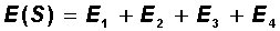
The first three components are responsible for the admissibility of the route: each city must be visited no more than once (there is no more than one unit in each row of the matrix), no more than one city must be visited under each number (no more than one unit in each column) and besides, the total number of visits equals the number of cities N (there are exactly N units in the matrix of all):
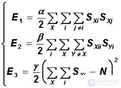
It can be seen that each of these three terms vanishes on valid routes, and takes values greater than zero to invalid. The last, fourth term minimizes the length of the route:

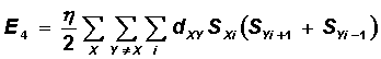
Here, d XY is the distance between cities X and Y. Note that the XY segment is included in the sum only when city Y is relative to city X, either the previous one or the next one. The factors a , b , g, and h have the meaning of the relative weights of the terms.
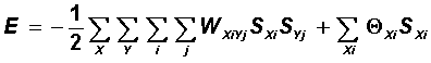
A general view of the Lyapunov function of the Hopfield network is given by the expression (see previous lecture):

The resulting objective function of the four terms is represented in the form of a Lyapunov function, if we choose the values of weights and thresholds of the network in the following form:
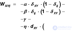
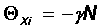
Now, it is possible to replace Hebb’s training with the direct assignment of the specified weights and thresholds for the neural network, and the dynamics of the resulting system will lead to a decrease in the length of the com-voyager route. In this problem, it is advisable to use probabilistic dynamics with simulated annealing, since the global minimum energy is of greatest interest.
Hopfield and Tancom described the model was tested in a computational experiment. The neural network managed to find close to optimal solutions for reasonable times, even for tasks with several dozens of cities. In the subsequent, many publications followed on various applications of neural network optimizers. At the end of the lecture, let us consider one of these applications - the problem of deciphering a character code.
Let there be some (rather long) text message written in a language using the alphabet A, B, C ... z and the space character responsible for the space between words. This message is encoded in such a way that each character, including a space, is associated with a certain character from the series i, j, k, .... It is required to decrypt the message.
This task also refers to the number of NP-complete, the total number of cipher keys has a factorial dependence on the number of characters in the alphabet. An approximate neural network solution can be based on the fact that the frequencies of occurrence of individual characters and specific pairs of characters in each language have quite specific meanings (for example, in Russian, the frequency of the appearance of the letter “a” significantly exceeds the frequency of the appearance of the letter “y”, the syllable “in "Appears quite often, but, for example, the combination" ysch "is not at all possible).
The frequency of occurrence of the symbols P i and their pairs P ij in the encoded message can be calculated directly. Having, further, at the disposal of the P A values of the frequencies of appearance of symbols of a language and their pairs P AB , it is necessary to identify them with the calculated values for the code. The best match will give the required key.
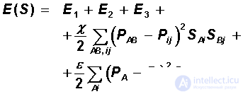
The objective function of this task contains five terms. The first three terms are sequentially the same as the first three terms in the expression for energy in the comiviary problem. They determine the admissibility of the key (each character of the language is associated with one character code). The remaining terms are responsible for the coincidence of the frequencies of individual symbols and the frequencies of pairs in the code and language.
The full expression for the objective function is:
The objective function, as well as for the task of the voyager, is reduced to the Lyapunov function, after which the neural network performs the required decoding.
1. By direct calculation, make sure that all the images of the training sample are stable states of a network with orthogonalization of the Hebb matrix.
2. For the task of the comivarius, get a representation E (S) of the objective function in the form of a Lyapunov function.
3. To derive the energy function of the Hopfield network for the problem of optimal placement of code and data mixtures in the hypercube multiprocessor architecture.
The decision (Terekhov SA, Oleynikov P.V., 1994). In a multiprocessor computer of this architecture, the processors are located at the vertices of a multidimensional cube. Each processor is connected to the nodes closest to it. Each processor is assigned a piece of program code and local data. В процессе вычислений процессоры обмениваются информацией, при этом скорость выполнения программ замедляется. Время, затрачиваемое на пересылку сообщения тем больше, чем дальше обменивающиеся процессоры расположены друг от друга.Требуется так разместить смеси кода и данных по реальным процессорам, чтобы максимально снизить потери на обмены информацией.
Как и в задаче комивояжера, обозначим процессоры заглавными буквами, а номера смесей - латинскими индексами. Если d XY - расстояние между процессорами, измеренное вдоль ребер гиперкуба (Хеммингово расстояние), а D ij - объем передаваемой информации между смесями i и j, то искомое решение должно минимизировать сумму SUM d XY D ij . Поэтому целевая функция представляется в виде:
This expression is further reduced to the form of the Lyapunov function. Numerical experiments with hypercubes of dimensions 3, 4 and 5 show that the use of the neural network approach allows one to obtain the knowledge of the number of information exchanges (and, accordingly, increase the computer performance) for some tasks up to 1.5 times.

Comments
To leave a comment
Computational Neuroscience (Theory of Neuroscience) Theory and Applications of Artificial Neural Networks
Terms: Computational Neuroscience (Theory of Neuroscience) Theory and Applications of Artificial Neural Networks