Lecture
ANN can be considered as a weighted directed graph in which artificial neurons are nodes. According to the architecture of connections, ANNs can be grouped into two classes (Fig. 5): forward-propagation networks, in which the graphs do not have loops, and recurrent networks, or networks with feedback.
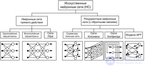
A RBF network (radial basis functions) is an artificial neural network that uses radial basis functions as activation functions.
ART - Adaptive Resonance Theory, Adaptive Resonance Networks is a kind of artificial neural networks based on the theory of adaptive resonance by Stephen Grossberg and Gale Carpenter. Includes models that use learning with a teacher and without a teacher and are used in solving problems of pattern recognition and prediction.
Neural networks are distinguished by:
· Network structure (connections between neurons);
· Features of the neuron model;
· Features of network training.
According to the structure, neural networks can be divided (Figure 8) into:
· Incomplete (or layered) and fully connected;
· With random and regular connections;
· With symmetric and asymmetrical connections.
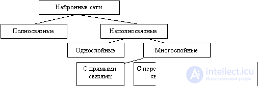
Figure 8 - Classification of neural networks by structure
The incompletely connected neural networks (described by a incompletely connected oriented graph and commonly called perceptrons) are subdivided into single-layer (simplest perceptrons) and multi-layered, with direct, cross-sectional and feedback connections . In neural networks with direct connections, the neurons of the j-th layer can only be connected via inputs to the neurons of the i-th layers, where j> i, i.e. with the neurons of the underlying layers. In neural networks with cross connections, connections within a single layer are allowed, i.e. the above inequality is replaced by j> = i. In neural networks with feedback, the j-th layer connections by inputs with i-th are used with j
In terms of topology, there are three main types of neural networks:
· Fully connected (Figure 9, a);
· Multilayer or layered (Figure 9, b);
· Weakly connected (with local connections) (Figure 9, c). 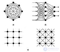
Figure 9 - Neural network architectures: a is a fully connected network, b is a multilayered network with serial connections, and c is weakly connected networks
In fully connected neural networks, each neuron transmits its output signal to the rest of the neurons, including itself. All input signals are given to all neurons. The output signals of the network can be all or some of the output signals of neurons after several cycles of network operation.
In multilayer neural networks, neurons are combined into layers. The layer contains a set of neurons with single input signals. The number of neurons in a layer can be any and does not depend on the number of neurons in other layers. In general, the network consists of Q layers, numbered from left to right. External input signals are fed to the inputs of the neurons of the input layer (it is often numbered as zero), and the network outputs are the output signals of the last layer. In addition to the input and output layers, there are one or more hidden layers in the multilayer neural network. Connections from the outputs of the neurons of some layer q to the inputs of the neurons of the next layer (q + 1) are called sequential.
In turn, the following types are distinguished among multilayered neural networks.
1) Monotone . This is a special case of layered networks with additional conditions for communication and neurons. Each layer except the last (output) is divided into two blocks: exciting and braking. Relations between the blocks are also divided into braking and exciting. If only excitatory connections are conducted from the neurons of block A to the neurons of block B, this means that any output signal of the block is a monotonous non-decreasing function of any output signal of block A. If these connections are only inhibitory, then any output signal of block B is a non-increasing function of any the output signal of block A. For neurons of monotone networks, a monotonic dependence of the output signal of the neuron on the parameters of the input signals is necessary.
2) Networks without feedback . In such networks, the neurons of the input layer receive input signals, transform them and transmit to the neurons of the first hidden layer, and so on up to the output, which outputs signals for the interpreter and the user. Unless otherwise stated, each output signal of the q-th layer will be fed to the input of all neurons of the (q + 1) -th layer; However, a variant of the connection of the q-th layer with an arbitrary (q + p) -th layer is possible.
Among the multilayer networks without feedback, there are distinguished fully connected (the output of each neuron of the q-th layer is connected with the input of each neuron of the (q + 1) -th layer) and partially fully connected. The classic version of layered networks are fully connected direct distribution networks (Figure 10).
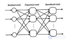
Figure 10 - Multi-layer (two-layer) network of direct distribution
3) Networks with feedback . In networks with feedback, information from subsequent layers is transmitted to previous ones. Among them, in turn, are the following:
· Layered cyclical , characterized in that the layers are closed in a ring: the last layer transmits its output signals to the first; all layers are equal and can both receive input signals and output the output;
· Layered fully connected consist of layers, each of which is a fully connected network, and the signals are transmitted both from layer to layer and inside the layer; in each layer, the work cycle is divided into three parts: receiving signals from the previous layer, exchanging signals inside the layer, generating an output signal, and transmitting to the next layer;
· Fully-layered , structurally similar to layered-fully-connected, but functioning differently: they do not separate the phases of exchange within the layer and transfer to the next, at each step neurons of all layers receive signals from neurons of both their layer and the subsequent ones.
As an example of feedback networks, Figure 11 shows the partially recurrent networks of Ellman and Jordan.
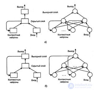
Figure 11 - Partially recurrent networks: a - Elman, b - Jordan
In loosely coupled neural networks, neurons are located at the nodes of a rectangular or hexagonal lattice. Each neuron is connected to four (von Neumann neighborhood), six (Golay neighborhood) or eight (Moore neighborhood) by its closest neighbors.
Known neural networks can be divided by type of neuron structure into:
· Homogeneous (homogeneous);
· Heterogeneous.
Homogeneous networks consist of neurons of the same type with a single activation function, and neurons with different activation functions enter a heterogeneous network .
Another classification divides neural networks into:
· Synchronous;
· Asynchronous.
In the first case, at each time point, only one neuron changes its state, in the second, the state changes immediately for a whole group of neurons, as a rule, for the entire layer. Algorithmically, the course of time in neural networks is given by iteratively performing similar actions on neurons.
According to the signals used at the inputs and outputs, neural networks can be divided into:
· Analog;
· Binary.
Binary operate only with binary signals, and the output of each neuron can take the value of either a logical zero (inhibited state) or a logical unit (excited state).
By time modeling, neural networks are divided into networks:
· With continuous time;
· With discrete time.
For software implementation, discrete time is usually applied.
By the method of presenting information to the inputs of a neural network, there are:
· Signaling at synapses of the input neurons;
· Giving signals to the outputs of the input neurons;
· Giving signals in the form of weights of synapses of input neurons;
· Additive feed to the synapses of the input neurons.
By the method of retrieving information from the outputs of the neural network are distinguished:
· I will eat from exits of output neurons;
· Removal from the synapses of the output neurons;
· I will pick up in the form of weights of synapses of output neurons;
· Additive removal from the synapses of the output neurons.
In terms of training organization, neural network training is divided into:
· With a teacher (supervised neural networks);
· Without a teacher (nonsupervised).
When training with a teacher, it is assumed that there is an external environment that provides training examples (input values and corresponding output values) at the training stage or evaluates the correct functioning of the neural network and changes the state of the neural network in accordance with its criteria or encourages (punishes) the neural network , thereby triggering a mechanism for changing its state.
According to the method of learning share learning:
· At the entrances
· On exits.
When learning by input, the learning example is only a vector of input signals, and when learning by outputs , it also includes the output signal vector corresponding to the input vector.
By way of presentation of examples distinguish:
· Presentation of single examples
· Presentation of the "page" of examples.
In the first case, the change in the state of the neural network (training) occurs after the presentation of each example. In the second - after the presentation of the "page" (set) of examples based on the analysis of all of them at once.
The state of the neural network, which may change, is usually understood as:
· Neuron synapse weights (weights map — map) (connectionist approach);
· Synapse weights and neuron thresholds (usually in this case, the threshold is more easily variable than the synapse weights);
· Establishing new connections between neurons (the ability of biological neurons to establish new connections and eliminate old ones is called plasticity).
According to the features of the neuron model, neurons with different non-linear functions are distinguished:
threshold 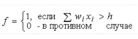 ;
;
Most often, the following sigmoid types are used as activation functions:
Fermi function (exponential sigmoid):

Rational sigmoid (with  = 0 degenerates into a so-called. threshold activation function):
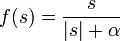
Hyperbolic Tangent:
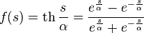 ,
,
where s is the output of the neuron adder, Is an arbitrary constant.
The listed functions refer to one-parameter.
Multiparameter transfer functions are also used, for example, 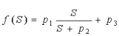 .
.
The most common models of neural networks:
· Hopfield model;
· Boltzmann machine;
· Kohonen network;
· Hamming model;
· Multilayer perceptron.
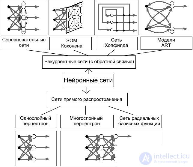
fig.5. Basic neural network architectures
Consider the basic terminology and understanding of what is happening in this area, from which building blocks of neural networks, and how to use it.
introduction about what a neuron is , a neural network , a deep neural network , so that we can communicate in the same language.
Then there are important trends that are happening in this area. Then we will look at the architecture of neural networks , we will consider their 3 main classes . Uh
After that, we will look at 2 relatively advanced topics and end with a small overview of the frameworks and libraries for working with neural networks.
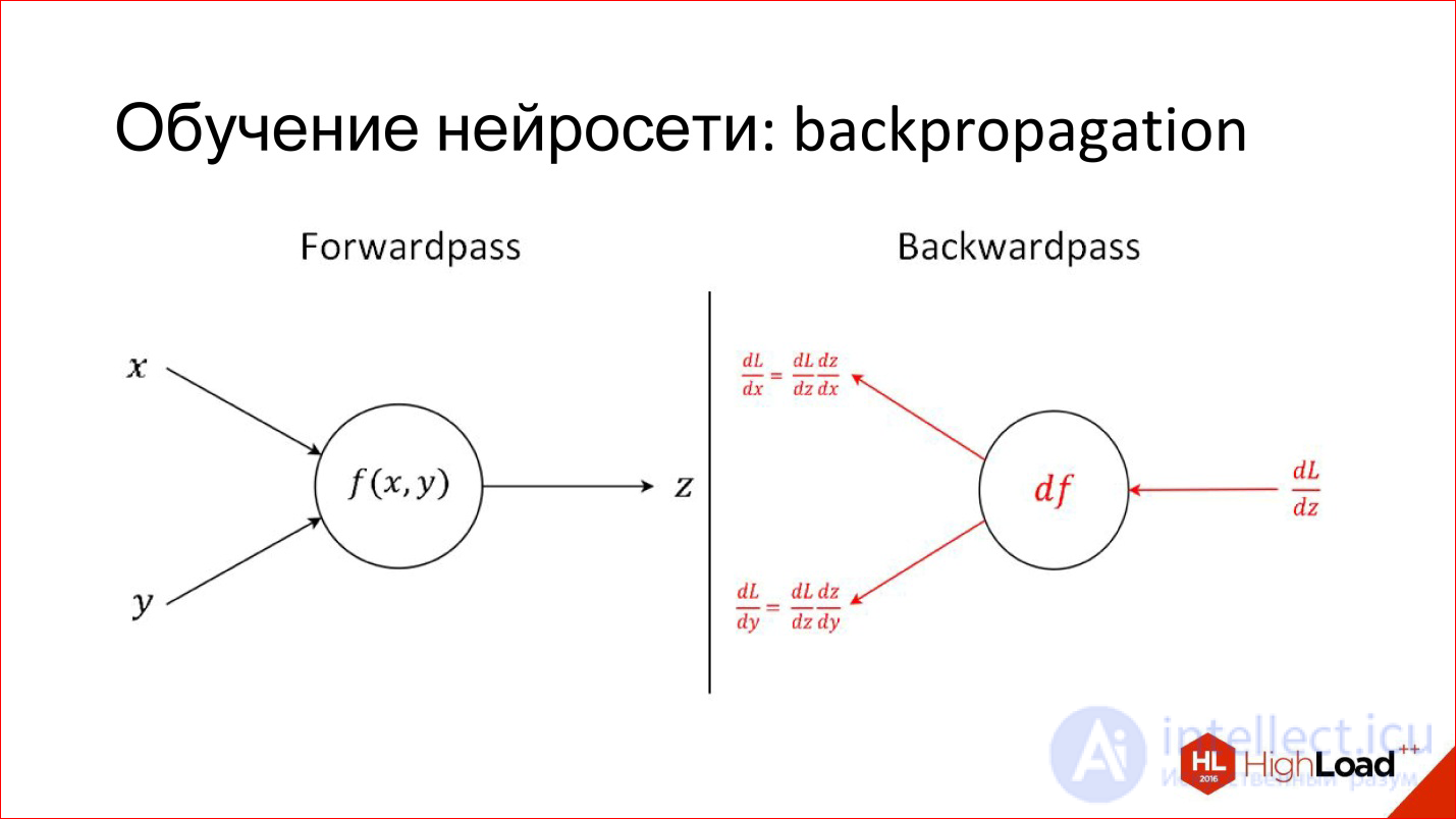
Another useful thing to know when discussing neural networks. I have already described how one neuron works: how each input multiplies by weights, by coefficients, sums up, multiplies by non-linearity. This is, let's say, the production mode of the neuron, that is, inference, as it works in the already trained form.
There is a completely different task - to train a neuron. Training is to find these correct weights. The training is based on the simple idea that if we, at the output of the neuron, know what the answer should be, and know how it turned out, we will know this difference, an error. This error can be sent back to all inputs of the neuron and understand what input influenced this error, and, accordingly, adjust the weight on this input so that the error is reduced.
This is the main idea behind Backpropagation, an error back-propagation algorithm. This process can be driven throughout the network and for each neuron to find how its weight can be modified. For this you need to take derivatives, but in principle, recently it is not required. All packages for working with neural networks are automatically differentiated. If 2 years ago it was necessary to manually write complex derivatives for tricky layers, now the packages do it themselves.
What is happening with the quality and complexity of models
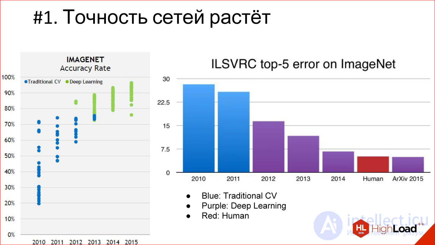
Firstly, the accuracy of neural networks is growing, and is growing very strongly. There are already a few examples when neural networks come to some area and force out the whole classical algorithm. So it was in image processing and speech recognition, it will happen in different areas. That is, there are neural networks that greatly reduce the error.
Deep Learning is highlighted in purple on the diagram, and the classic computer vision algorithm is highlighted in blue. It is seen that Deep Learning has appeared, the error has decreased and continues to decrease further. That is why Deep Learning completely supersedes all, conditionally, classical algorithms.
Another important milestone is that we are beginning to overtake the quality of a person. At the ImageNet competition, this happened for the first time in 2015. But in fact, neural network systems that are superior to humans in quality have appeared earlier. The first documented distinct case is 2011, when a system was built that recognized German road signs and did it 2 times better than a person.
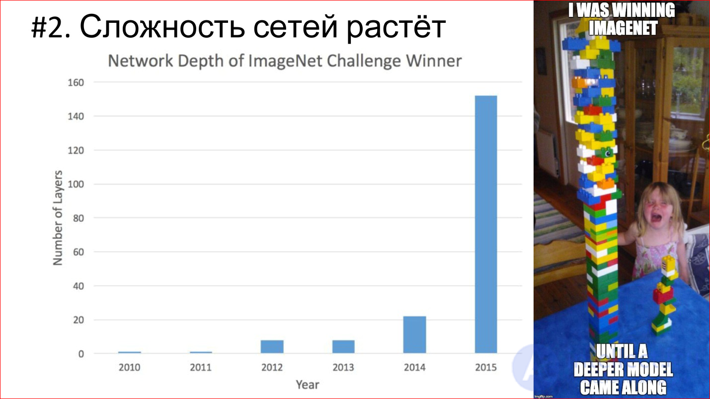
The second important trend - the complexity of neural networks is growing. In terms of depth, depth increases. If the winner of 2012 on ImageNet is the AlexNet network - there were less than 10 layers, then in 2014 there were already more than 20, in 2015 - under 150. This year, it seems, already beyond 200. What will happen next is not clear, perhaps will be even more.

http://cs.unc.edu/~wliu/papers/GoogLeNet.pdf
In addition to the growing depth, the architectural complexity grows as well. Instead of simply joining the layers one by one, they begin to branch, blocks and structure appear. In general, the architectural complexity is also growing.
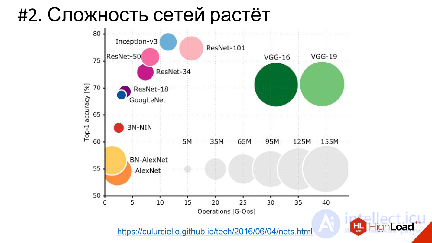
https://culurciello.github.io/tech/2016/06/04/nets.html
This is a graph of the accuracy of various neural networks. Here is the time it takes to execute, on the miscalculation of this network, that is, some computational load. The size of the circle is the number of parameters that are described by the neural network. It is interesting to compare the classic network AlexNet - the winner of 2012 and later networks. They are better in accuracy, but usually contain fewer parameters. This is also an important trend that neural networks complicate very cleverly. That is, the architecture changes so that even though the number of layers is 150, the total number of parameters is less than in the 6-7-layer network, which was in 2012. The architecture is somehow complicated in a very interesting way.
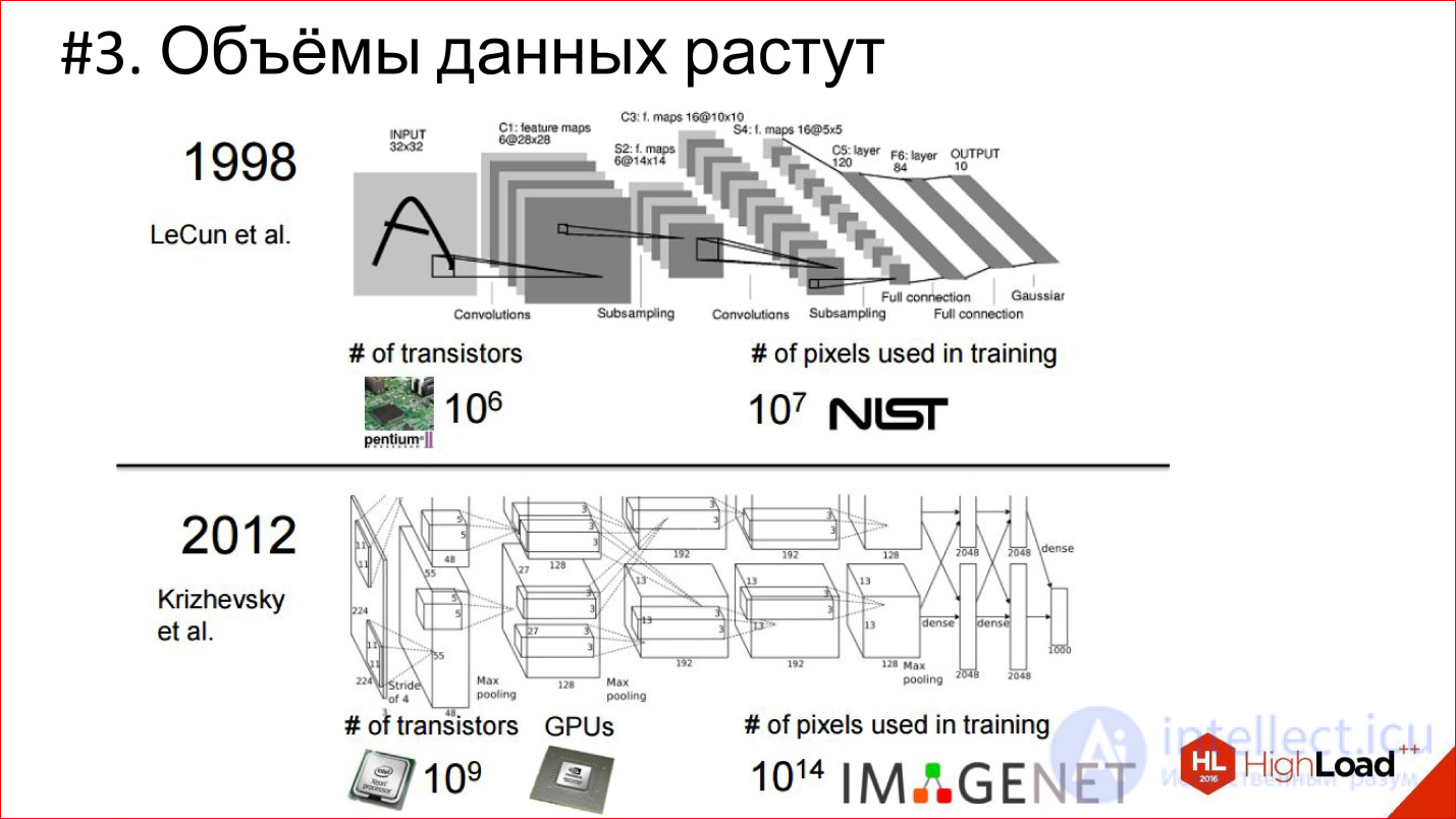
Another trend is data growth. In 1998 for training convolutional
The neural network that recognized the handwritten checks was used 10 7 pixels, in 2012 (IMAGENET) - 10 14.
7 orders in 14 years is a crazy difference and a huge shift!
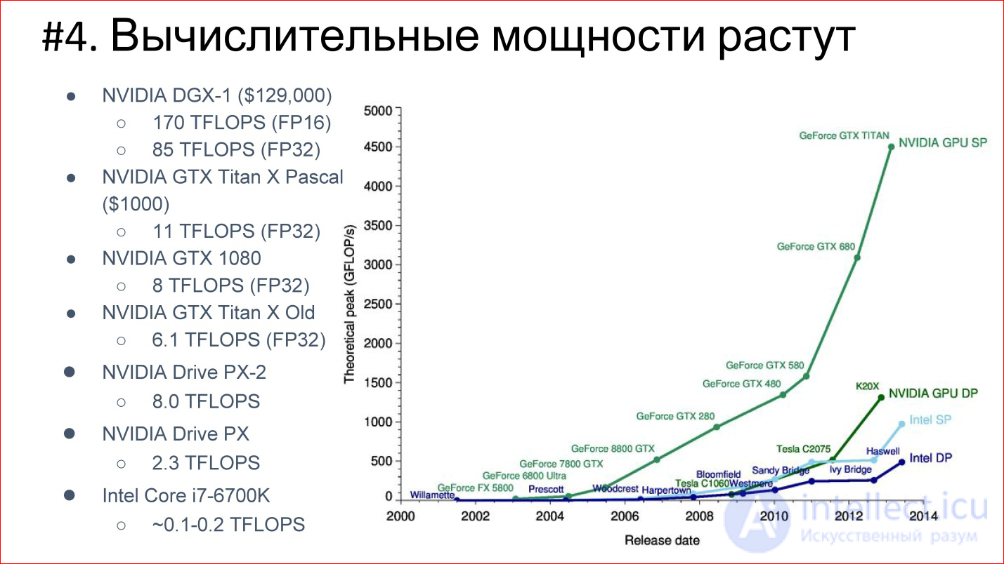
At the same time, the number of transits on the processor is also growing, computing power is growing - Moore's law is in effect. Over these 14 years, processors have become conditionally 1000 times faster. This is illustrated by the example of GPUs, which now dominate in the area of Deep Learning. Almost everything counts on graphics accelerators.
NVIDIA has been redeveloped from gaming to actually a company for artificial intelligence. Its exhibitors left far behind Intel exhibitors, which do not look at all against this background.
This is a picture of 2013, when the top-end video card was 4.5 TFLOPS. Now the new TITAN X is already 11 TFLOPS. In general, the exhibitor continues!
In fact, we can expect that FPGAs will appear in the near future, which will partially press the GPU, and maybe even neuromorphic processors will appear over time. Watch this - there is also a lot of interesting things happening.
Fully Connected Feed-Forward Neural Networks, FNN
The first classical architecture is fully connected direct propagation neural networks, or Fully Connected Feed-Forward Neural Network, FNN.
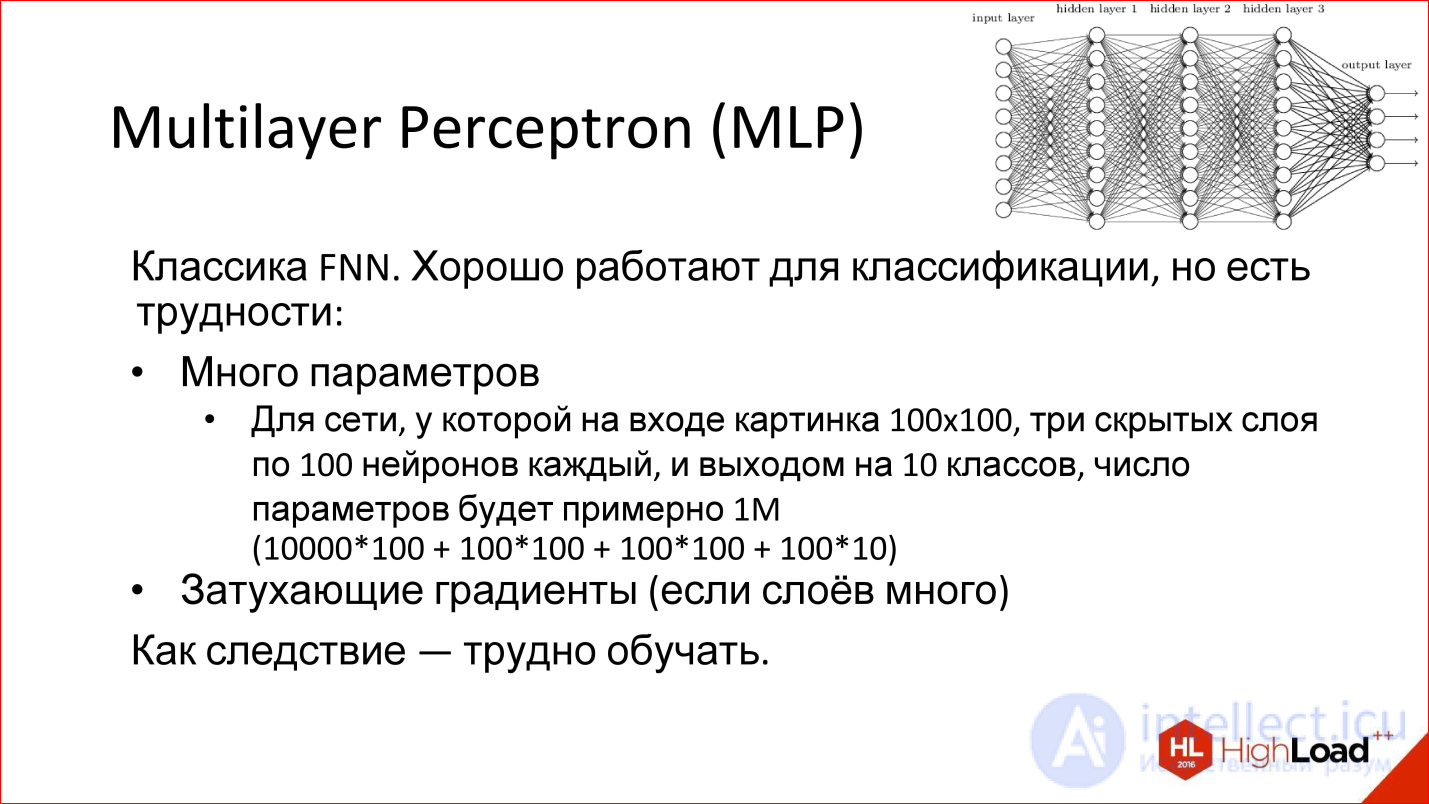
Multi-layer Perceptron is generally a neural network classic. That picture of neural networks that you saw, this is it - a multilayered fully connected network. Full connected - this means that each neuron is connected with all the neurons of the previous layer. A good network works, it is suitable for classification, many classification problems are successfully solved.
However, she has 2 problems:
For example, if you take a neural network of 3 hidden layers that needs to process 100 * 100 ps pictures, this means that there will be 10,000 ps at the input, and they are added to 3 layers. In general, to be honest with all the parameters, such a network will have about a million. It really is a lot. To train a neural network with a million parameters, you need a lot of training examples that are not always there. In fact, there are examples now, but they were not there before - therefore, in particular, the networks could not train as they should.
In addition, the network, which has many parameters, has an additional tendency to retrain. It can be sharpened by something that in reality does not exist: some noise Data Set. Even if, in the end, the network remembers examples, but on those that it did not see, then it will not be able to be used normally.
Plus there is another problem called:
Remember that story about Backpropagation, when an error from the outputs is sent to the input, distributed to all weights and sent further along the network? Further, these derivatives - that is, the gradient (error derivative) - are run back through the neural network. When there are many layers in a neural network, a very, very small part of this gradient can remain at the very end. In this case, the input weight will be almost impossible to change because this gradient is practically “dead”, it is not there.
This is also a problem, due to which deep neural networks are also difficult to train. We will return to this topic further, especially on recurrent networks.
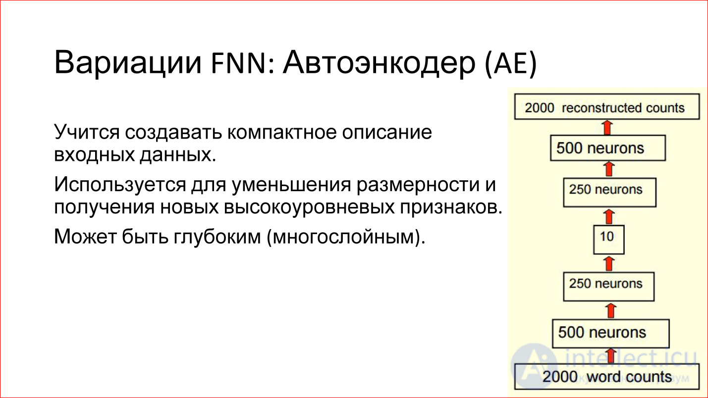
There are various variations of FNN networks. For example, a very interesting variation of the Auto ENCODER. This is a network of direct distribution with the so-called bottleneck in the middle. This is a very small layer, say, of only 10 neurons.
What are the advantages of such a neural network?
The purpose of this neural network is to take some kind of input, drive it through itself and generate the same input at the output, that is, so that they match. What's the point? If we can train such a network that takes input, drives it through itself and generates exactly the same output, it means that these 10 neurons in the middle are enough to describe this input. That is, you can greatly reduce the space, reduce the amount of data, economically encode any input data in the new terms of 10 vectors.
It is convenient and it works. Such networks can help you, for example, reduce the dimension of your task or find some interesting features that you can use.

There is another interesting model of RBM. I wrote it in the FNN variation, but in reality this is not true. Firstly, it is not deep, and secondly, it is not Feed-Forward. But it is often associated with FNN networks.
What it is?
This is a shallow model (on the slide it is drawn in a corner), which has an entrance and there is some hidden layer. You give a signal to the input and try to train the hidden layer so that it generates this input.
This is a generative model. If you have trained it, then you can generate analogs of your input signals, but slightly different. It is stochastic, that is, every time it will generate something slightly different. If you, for example, have trained such a model to generate handwritten ones, then it will accumulate them a number of slightly different ones.
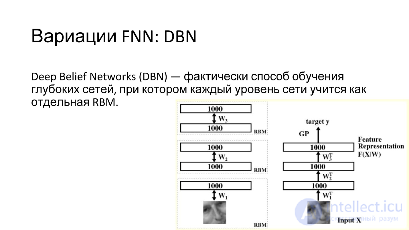
What is good about RBM is that they can be used to train deep networks. There is such a term — Deep Belief Networks (DBN) —in fact, this is a way to train deep networks, when 2 lower layers of a deep network are taken separately, input is given and RBM is trained on these first two layers. After that, these weights are recorded. Next, the second layer is taken, considered as a separate RBM and is also being trained. And so throughout the network. Then these RBMs are joined, combined into one neural network. It turns out a deep neural network, which should be.
But now there is a huge advantage - if earlier you had just taught it from some random (random) state, now it is not random — the network is trained to restore or generate data from the previous layer. That is, her weight is reasonable, and in practice this leads to the fact that such neural networks are already quite well trained. Then you can slightly train them with some examples, and the quality of such a network will be good.
Plus there is an additional advantage. When you use RBM, you essentially work on unallocated data, which is called Un supervised learning. You have just pictures, you do not know their classes. You drove millions, billions of pictures that you downloaded from Flickr or from somewhere else, and you have some kind of structure in the network itself that describes these pictures.
You do not know what it is yet, but these are reasonable weights, which can then be taken and supplemented by a small number of different pictures, and this will be good. This is a cool way to use a combination of 2 neural networks.
Then you will see that this whole story is really about Lego. That is, you have separate networks - recurrent neural networks, some other networks are all blocks that can be combined. They are well combined on different tasks.
These were the classic direct propagation neural networks. Next, we turn to convolutional neural networks.
Convolutional Neural Networks, CNN
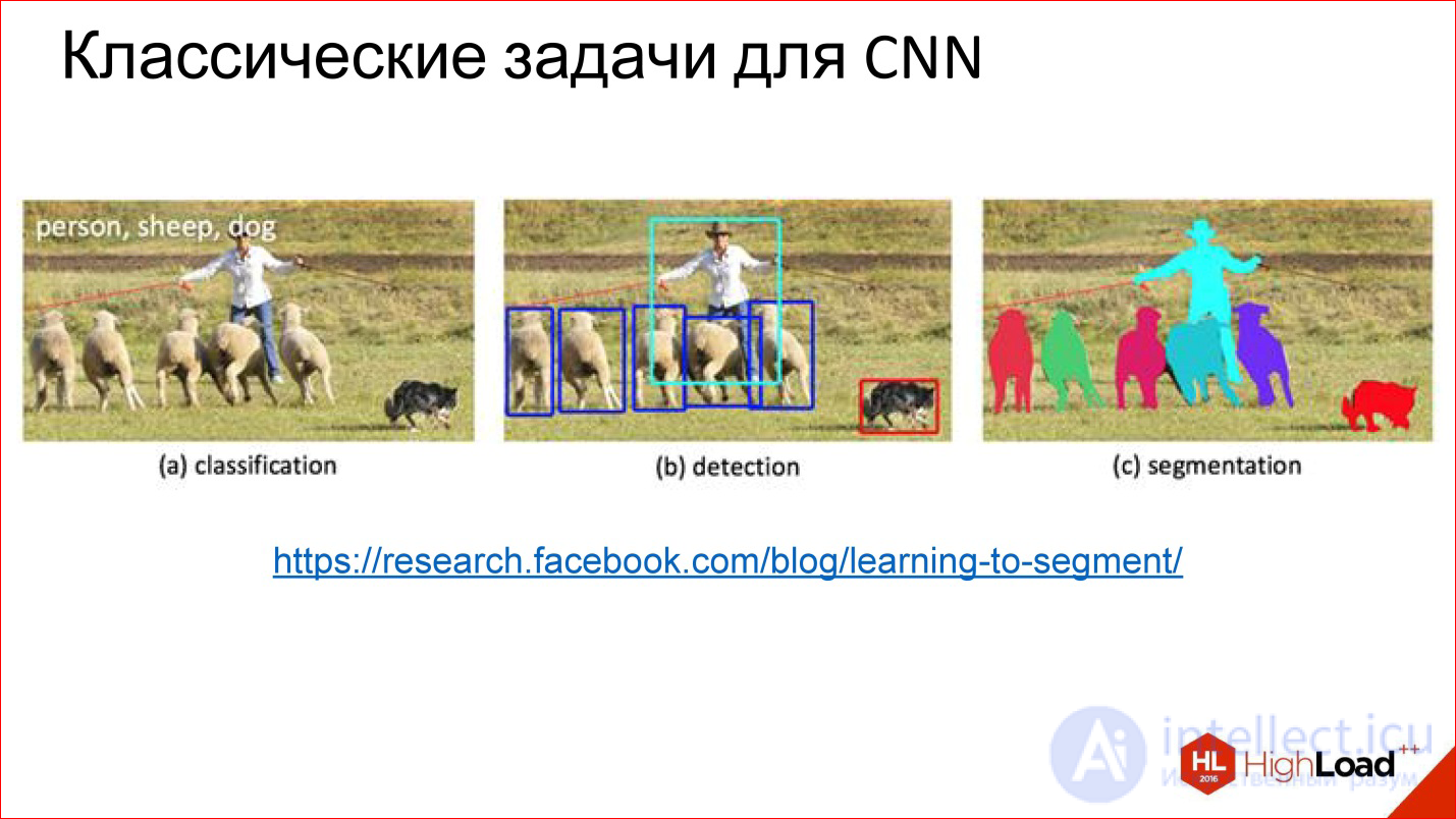
https://research.facebook.com/blog/learning-to-segment/
Convolutional neural networks solve 3 main tasks:
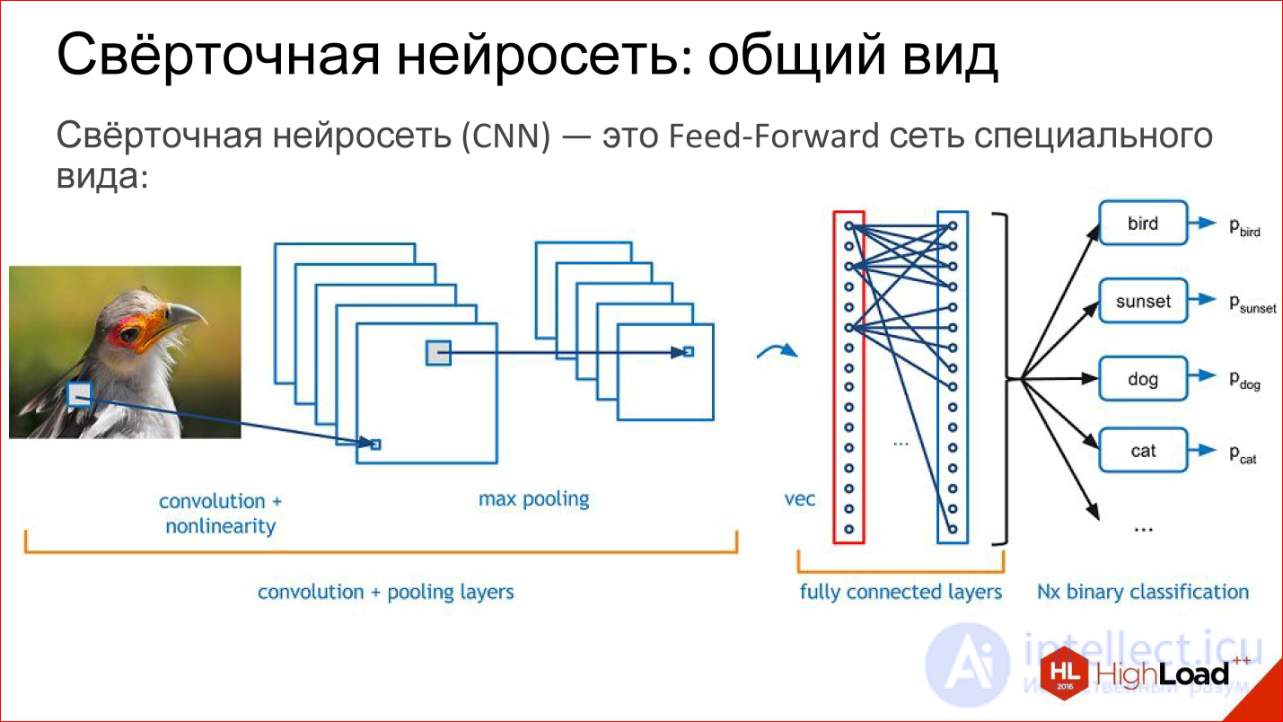
What is a convolutional neural network? In fact, the convolutional neural network is the usual feed-forward network, it’s just a little bit of a special kind. Lego starts now.
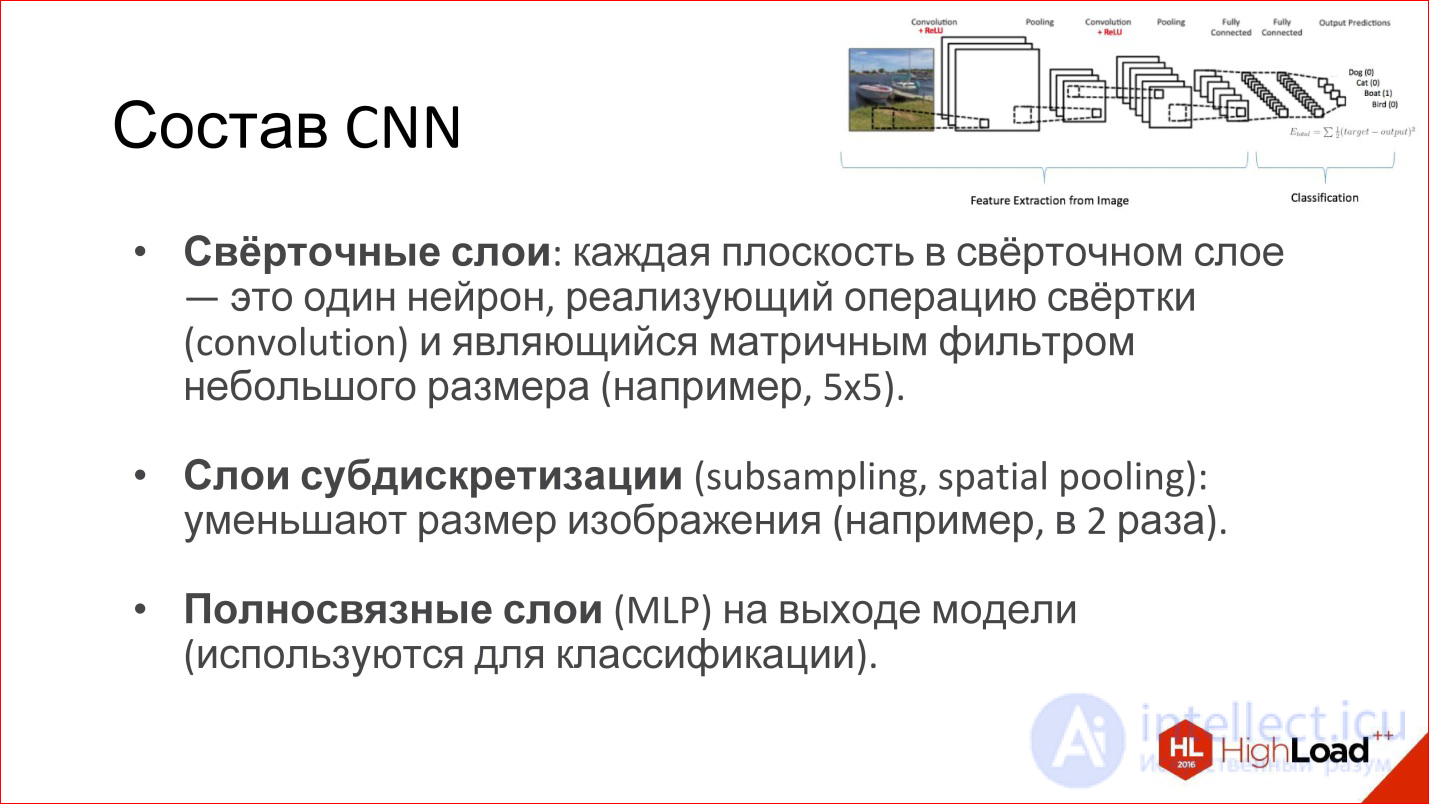
What is in the convolution network? She has:
A little more detail about all these layers.
http://intellabs.github.io/RiverTrail/tutorial/
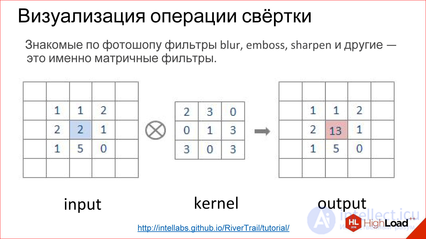
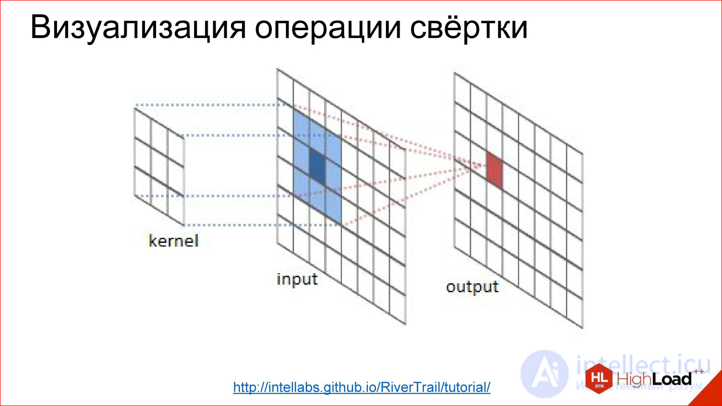
What is a convolution operation? It scares everyone, but in reality it’s a very simple thing. If you worked in Photoshop and made Gaussian Blur, Emboss, Sharpen and a bunch of other filters, these are all matrix filters. Matrix filters are in fact a convolution operation.
How is it implemented? There is a matrix, which is called the filter kernel (in the figure kernel). For Blur it will be all units. There is an image. This matrix is superimposed on a piece of the image, the corresponding elements are simply multiplied together, the results are added and recorded at the center point.
http://intellabs.github.io/RiverTrail/tutorial/
So it looks more clearly. There is an image Input, there is a filter. You run a filter over the entire image, honestly multiply the corresponding elements, add, write to the center. Run, run - built a new image. All this is a convolution operation.
That is, in fact, convolution in convolutional neural networks is a cunning digital filter (Blur, Emboss, anything else), which itself is trained.
http://cs231n.github.io/convolutional-networks/
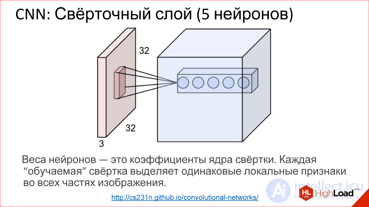
In fact, convolutional layers all work on volumes. That is, even if you take an ordinary RGB image, there are already 3 channels - this is, in fact, not a plane, but a volume of 3, conditionally, cubes.
Convolution in this case is no longer a matrix, but a tensor - actually a cube.
You have a filter, you run through the entire image, it immediately looks at all 3 color layers and generates one new point for one of this volume. Run through the entire image - built one channel, one plane of the new image. If you have 5 neurons, you have built 5 planes.
This is how the convolutional layer works. The task of learning the convolutional layer is the same as in ordinary neural networks - to find the weights, that is, to actually find the convolution matrix, which is completely equivalent to the weights in the neurons.
What are these neurons doing? They actually learn to look for some features, some local signs in the small part that they see - and that’s all. Running one such filter is building a certain map of finding these features in the image.
Then you built many such planes, then use them as an image, feeding them on the following entrances.
http://vaaaaaanquish.hatenablog.com/entry/2015/01/26/060622
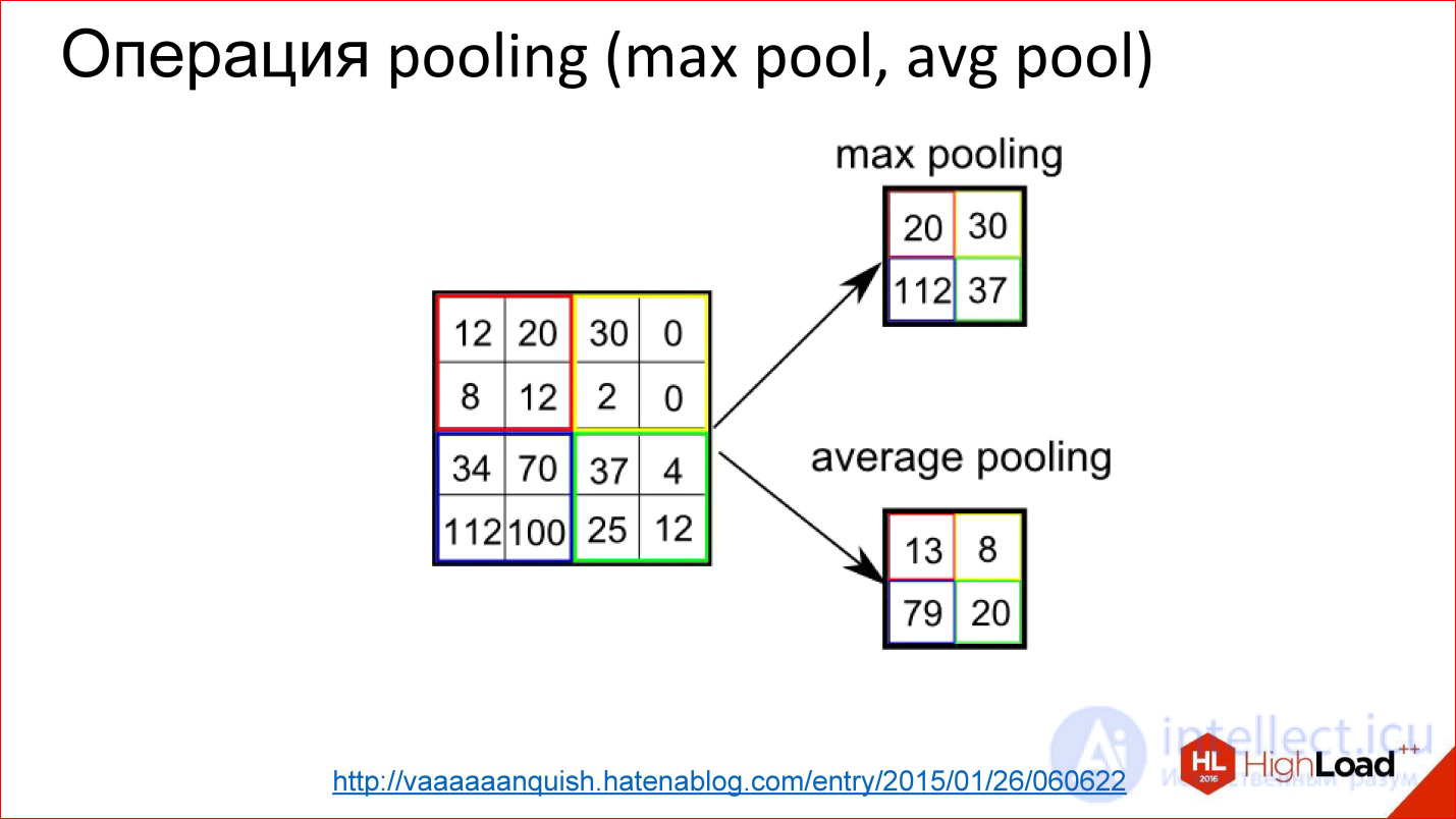
Pooling operation is an even simpler operation. It is just averaging or taking a maximum. It also works on some small squares, for example, 2 * 2. You overlay the image and, for example, select the maximum element from this 2 * 2 box, send it to the output.
Thus, you reduced the image, but not with a cunning Average, but with a slightly more advanced piece - you took the maximum. This gives a slight shift invariance. That is, it does not matter to you whether some sign was found in this position or 2 ps to the right. This thing allows the neural network to be a little more resistant to image shifts.
http://cs231n.github.io/convolutional-networks/
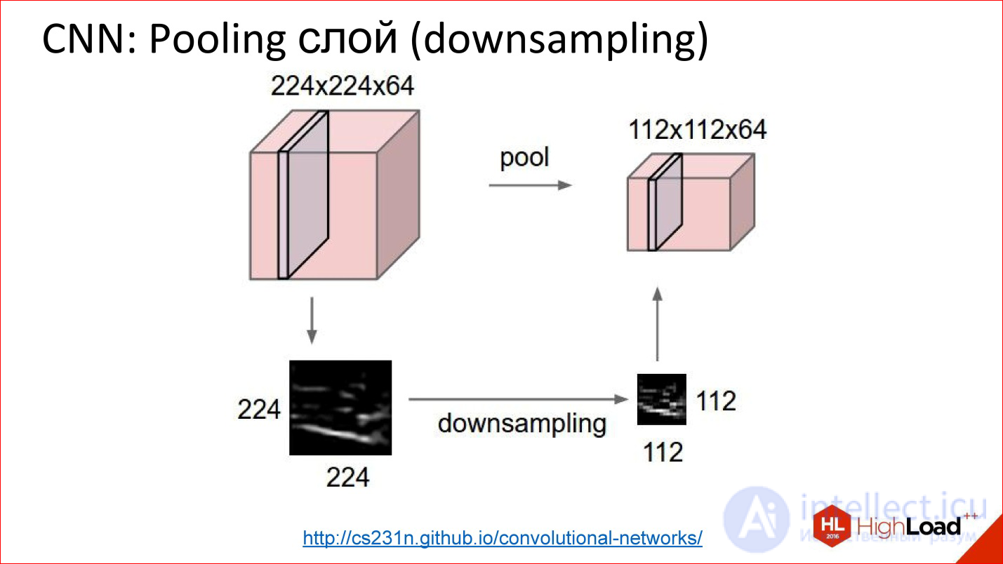
This is how the pooling layer works. There is a cube of some size - 3 channels, 10, or 100 channels, which you counted by convolutions. It simply reduces it in width and height, it does not touch the other dimensions. Everything is a primitive thing.
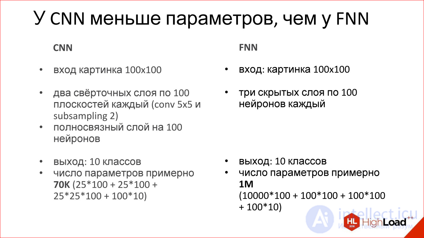
What are good convolutional networks?
They are good because they have much fewer parameters than a regular fully connected network. Remember the example of a fully connected network, which we considered, where we got a million weights. If we take a similar one, more precisely, a similar one — it cannot be called a similar one, but a close convolutional neural network, which has the same input, the same output, will also have one fully connected output layer and 2 more convolutional layers, where there will also be 100 neurons each. in the core network, it turns out that the number of parameters in such a neural network has decreased by more than an order of magnitude.
It's great if the parameters are so much smaller - the network is easier to train. We see it, it’s really easier to train.
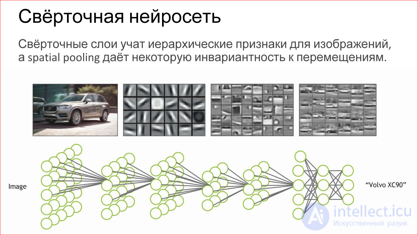
What does the convolutional neural network do?
In fact, it automatically learns some hierarchical features for images: first, basic detectors, lines of different inclination, gradients, etc. Of these, she collects some more complex objects, then even more complex ones.
If you perceive a neuron as a simple logistic regression, a simple classifier, then a neural network is just a hierarchical classifier. First, you single out simple signs, combine complex signs of them, even more complex ones, even more complex ones, and in the end you can combine some very complex sign - a specific person, a specific machine, an elephant, anything else.
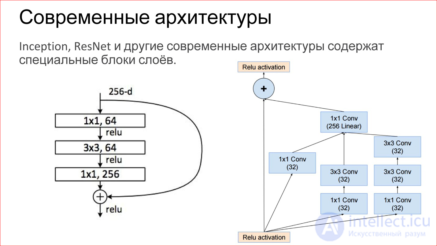
Modern architectures of convolutional neural networks have become very complicated. Those neural networks that won at the latest ImageNet contests are no longer just some convolutional layers, Pooling layers. These are directly finished blocks. The figure shows examples from the network Inception (Google) and ResNet (Microsoft).
In essence, the same basic components are inside: the same convolutions and pooling. Just now there are more of them, they are somehow slyly combined. Plus, now there are direct links that allow you not to transform the image at all, but simply transfer it to the output. It, by the way, helps that gradients do not fade. This is an additional way to pass the gradient from the end of the neural network to the beginning. It also helps to train such networks.
It was quite classic convolutional neural networks. Yes, there are different types of layers that can be used for classification. But there are more interesting uses.
https://arxiv.org/abs/1411.4038
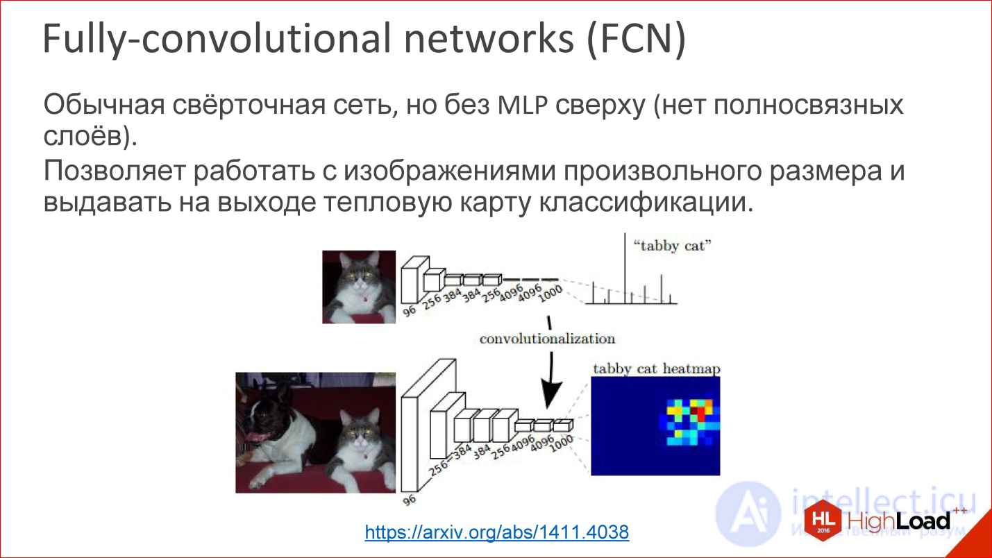
For example, there is such a kind of convolutional neural networks called Fully-convolutional networks (FCN). People rarely talk about them, but this is a cool thing. You can take and tear off the last multilayer perceptron, it is not needed - and throw it out. And then the neural network can magically work on images of arbitrary size.
That is, she learned, let's say, to define 1000 classes in the images of cats, dogs, something else, and then we took the last layer and did not tear it off, but transformed it into a convolutional layer. There are no problems - you can count the weights. Then it turns out that this neural network seems to work with the same window for which it was trained, 100 * 100 ps, but now it can run through this window across the entire image and build a heat map at the output - where in this particular image is specific class.
You can build, for example, 1000 of these Heatmap for all your classes and then use it to determine the location of the object in the picture.
This is the first example where a convolutional neural network is not used for classification, but in fact for generating an image.
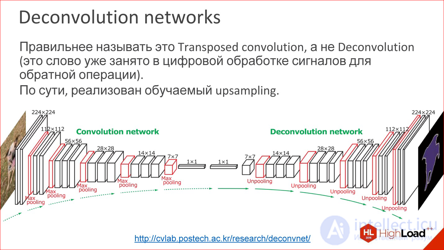
http://cvlab.postech.ac.kr/research/deconvnet/
A more advanced example is Deconvolution networks. They are rarely spoken of either, but this is even more awesome.
In fact, Deconvolution is the wrong term. In digital signal processing, this word is taken by a completely different thing - a similar, but not such.
What it is? In essence, it is a trained upsling. That is, at some point you have reduced your image to a small size, maybe even 1 ps. Rather, not to a pixel, but to some small vector. Then you can take this vector and open.
Or, if at some point you got an image of 10 * 10 ps, now you can do Upsampling of this image, but in some tricky way in which Upsampling weights are also trained.
This is not magic, it works, and in fact it allows us to train neural networks that receive some kind of output image from the input image. That is, you can submit entry / exit samples, and the one in the middle will learn by itself. It is interesting.
In fact, many tasks can be reduced to the generation of images. Classification is a cool task, but it is still not comprehensive. There are many tasks where pictures need to be generated. Segmentation is basically a classic task, where you need to have a picture at the output.
Moreover, if you have learned to do so, then you can do it in a different way, more interesting.
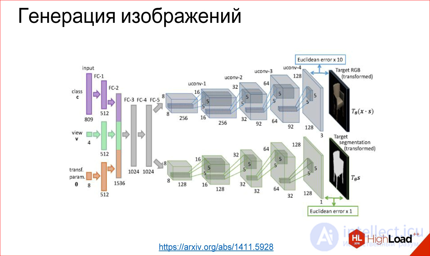
https://arxiv.org/abs/1411.5928
It is possible to tear off the first part, for example, and fasten some kind of fully meshed network that we will teach - what comes to the entrance, for example, a class number: generate a chair for me at such and such an angle and in such and such form. These layers generate further some internal representation of this chair, and then it unfolds into a picture.
This example is taken from the work where the neural network really taught to generate different chairs and other objects. It also works, and it's fun. This is collected, in principle, from the same basic blocks, but they are wrapped differently.

https://arxiv.org/abs/1508.06576
There are non-classical tasks, for example, the transfer of style, about which in the last year we all hear. There are a bunch of applications that can do this. They work on about the same technology.
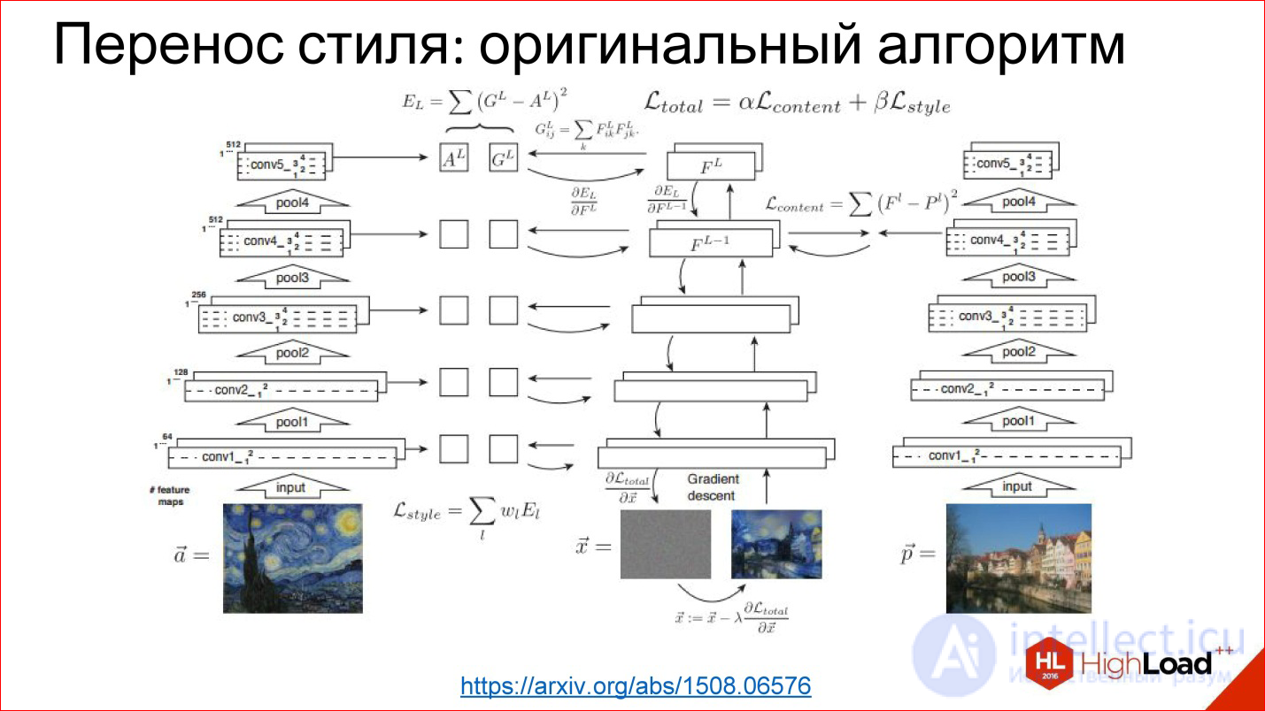
https://arxiv.org/abs/1508.06576
There is a ready trained network for classification. It turned out that if we take a derived picture, load it into this neural network, then different convolutional layers will be responsible for different things. That is, on the first convolutional layers there will be stylistic features of the image, on the latter - content features of the image, and this can be used.
You can take a picture as a model of style, drive it through a ready-made neural network, which was not taught at all, remove stylistic signs, remember. You can take any other picture, get rid of, take the content signs, remember. And then the random image (noise) can be driven away again through this neural network, to get the signs on the same layers, to compare with those that should have been received. And you have a task for Backpropagation. In fact, further gradient descent can be transformed random image to one for which these weights on the desired layers will be as necessary. And you got a stylized picture.
The only problem with this method is that it is long. This iterative run of the picture back and forth is a long time. Who played with this code in the style generation, knows that the classic code is long, and you have to suffer. All services like Prism and so on, which generate more or less quickly, work differently.
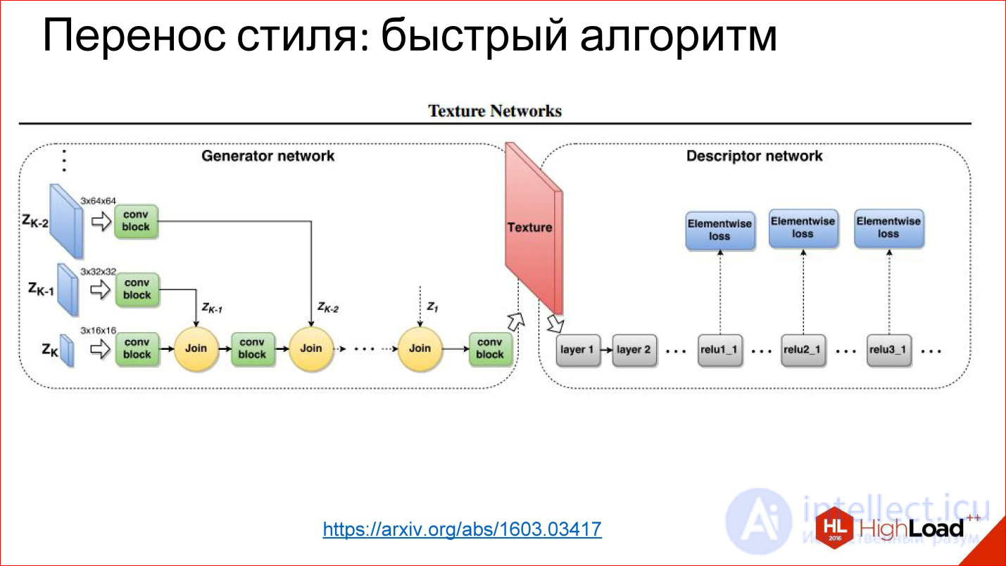
https://arxiv.org/abs/1603.03417
Since then, they have learned to generate networks that simply generate a picture in 1 pass. This is the same task of transforming an image that you have already seen: there is something at the entrance, there is something at the output, you can train everything in the middle.
In this case, the trick is that the loss function is the very function of the error you get on this neural network, and the error function is removed from the normal neural network that was trained for classification.
These are such hacker methods of using neural networks, but it turned out that they work, and this leads to cool results.
Next, we turn to recurrent neural networks.
Recurrent Neural Networks, RNN
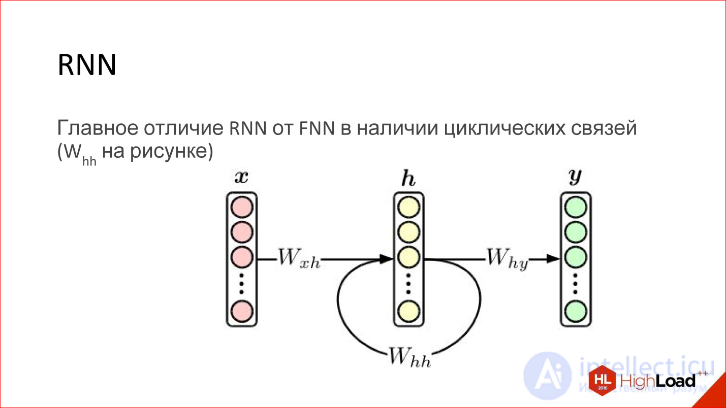
A recurrent neural network is actually a very cool thing. At first glance, their main difference from conventional FNN networks is that some kind of cyclic connection just appears. That is, the hidden layer sends its own values to itself in the next step. It would seem to be a minor thing, but there is a fundamental difference.
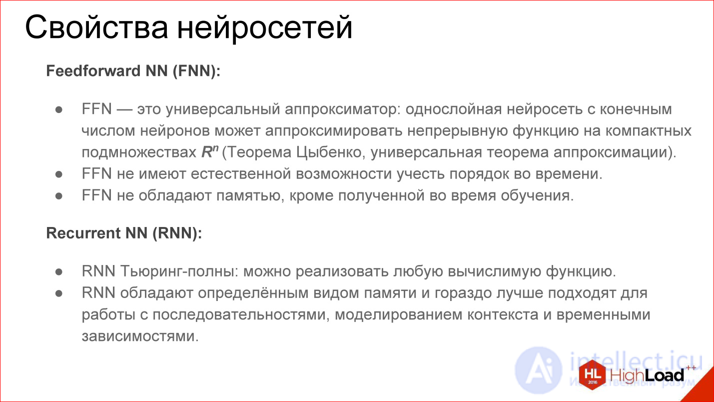
About the usual Feed-Forward neural network it is known that it is a universal approximator. They can approximate more or less any continuous function (there is such a Tsybenko theorem). It's great, but recurrent neural networks are turing full. They can calculate any computable.
Essentially, recurrent neural networks are a regular computer. The task is to train him correctly. Potentially, it can read any algorithm. Another thing is that it is difficult to teach him.
In addition, the usual Feed-Forward neural networks have no opportunity to take into account the order in time - this is not in them, not presented. Recurrent networks do this explicitly, the concept of time is embedded in them.
Regular feed-forward networks do not have any memory, except for the one that was obtained at the training stage, and recurrent networks do. Due to the fact that the content of the layer is transferred back to the neural network, it is like its memory. It is stored while the neural network is running. This also adds a lot.
http://colah.github.io/posts/2015-08-Understanding-LSTMs/
How are recurrent neural networks trained? In fact, almost the same. In addition to Backpropagation, of course, there are many other algorithms, but at the moment Backpropagation works best.
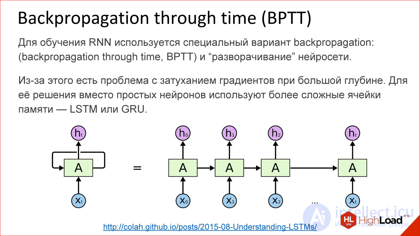
For recurrent neural networks, there is a variation of this algorithm - Backpropagation through time. The idea is very simple - you take a recurrent neural network and the cycle simply expands on a few steps, for example, 10, 20 or 100, and you get an ordinary deep neural network, which you then teach with ordinary Backpropagation.
But there is a problem. As soon as we start talking about deep neural networks - where there are 10, 20, 100 layers - there is nothing left from the gradients that should pass to the very beginning from the end, there are no 100 layers. With this we need to do something. In this place a certain hack was invented, a beautiful engineering solution called LSTM or GRU is the memory cells.
https://deeplearning4j.org/lstm
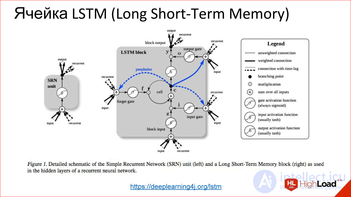
Their idea is that the visualization of a normal neuron is replaced by some kind of clever thing that has memory and there is a gate, which control when this memory needs to be reset, rewritten or saved, etc. These gates are also trained in the same way as everything else. In fact, this cell, when it has learned, can tell the neural network that we are now keeping this internal state for a long time, for example, 100 steps. Then, when the neural network used this state for something, it can be reset. It became unnecessary, we went to a new count.
On all more or less serious tests, these neural networks strongly do the usual classical recurrent ones, which are simply on neurons. Almost all recurrent networks are currently built on either LSTM or GRU.

http://kvitajakub.github.io/2016/04/14/rnn-diagrams
I will not go into what it is inside, but these are such tricky blocks, much more complicated than ordinary neurons, but, in fact, they are similar. There are some gateways that control this very “remember - do not remember”, “pass on - do not pass on”.
These were the classic recurrent neural networks. Then begins the topic, which is often silent, but it is also important.
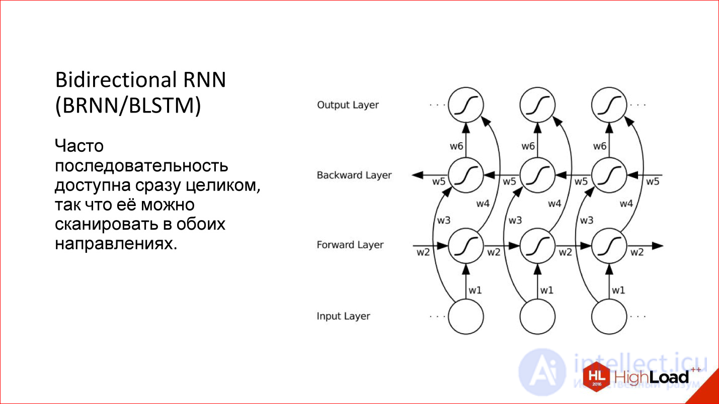
When we work with a sequence in a recurrent network, we usually feed one element, then the next, and set the previous state of the network to the input, this natural direction arises - from left to right. But it is not the only one! If we have, for example, a proposal, we begin to submit his words in the usual way to the neural network - yes, this is the normal way, but why not submit it from the end?
That is, in many cases, the sequence has been given entirely from the very beginning. We have this proposal, and it makes no sense to somehow single out one direction relative to another. We can run a neural network on the one hand, on the other hand, actually having 2 neural networks, and then combine their result.
This is called Bidirectional - a bi-directional recurrent neural network. Their quality is even higher than conventional recurrent networks, because there is more context: for each point there are now 2 contexts - what was before, and what will be after. For many tasks this adds quality, especially for language related tasks.
For example, there is German, where in the end something will definitely be hung up, and the sentence will change - such a network will help.
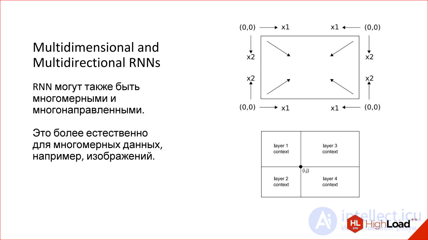
Moreover, we considered one-dimensional cases - for example, sentences. But there are multidimensional sequences - the same image can also be viewed as a sequence. Then he generally has 4 directions that are reasonable in their own way. For an arbitrary point of the image there are, in fact, 4 contexts with such a detour.
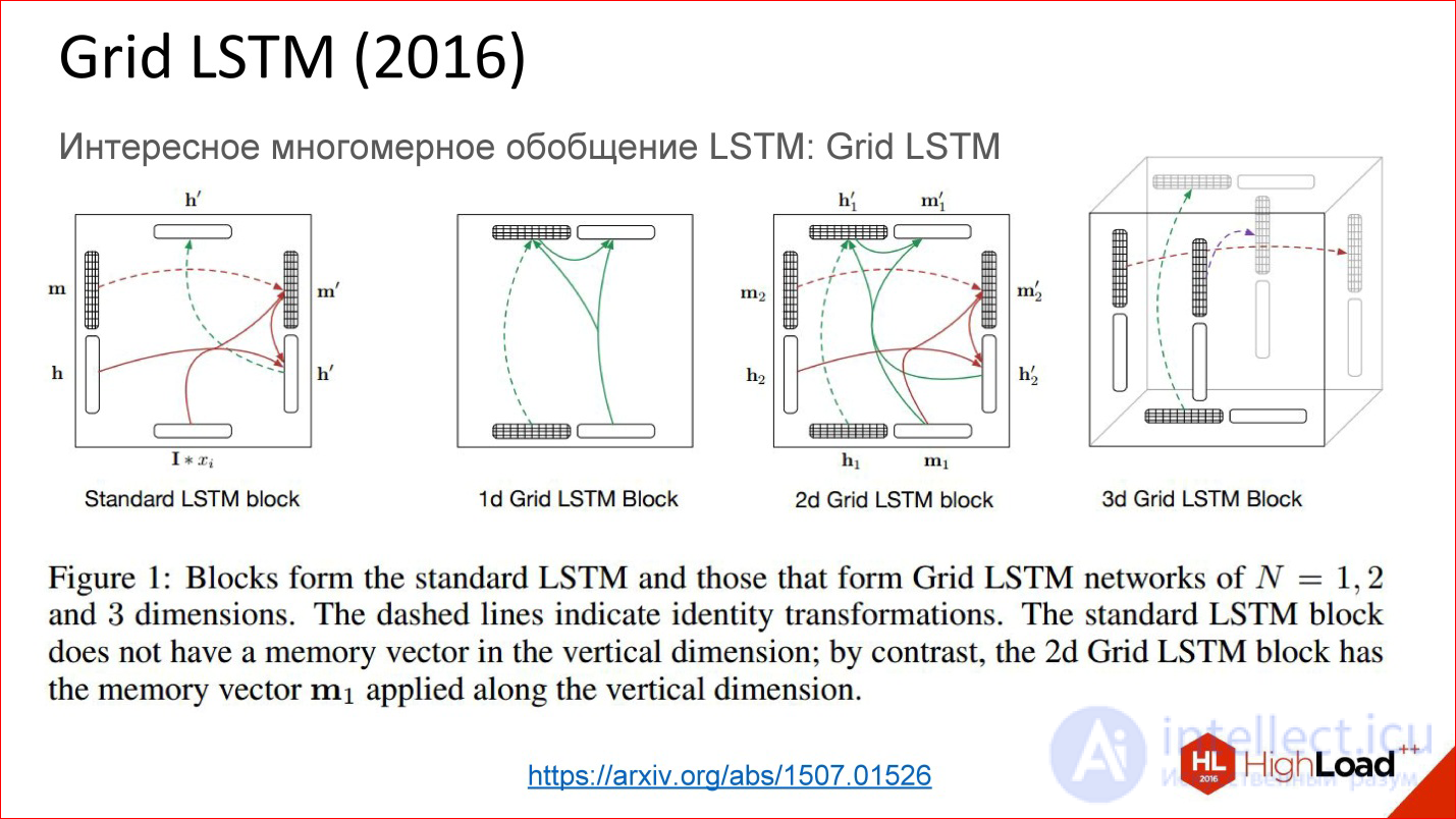
There are interesting multidimensional recurrent neural networks: they are both multidimensional and multidirectional. Now they are a little forgotten. This, by the way, is an old development, which is already 10 years old, probably, but now it is beginning to emerge.
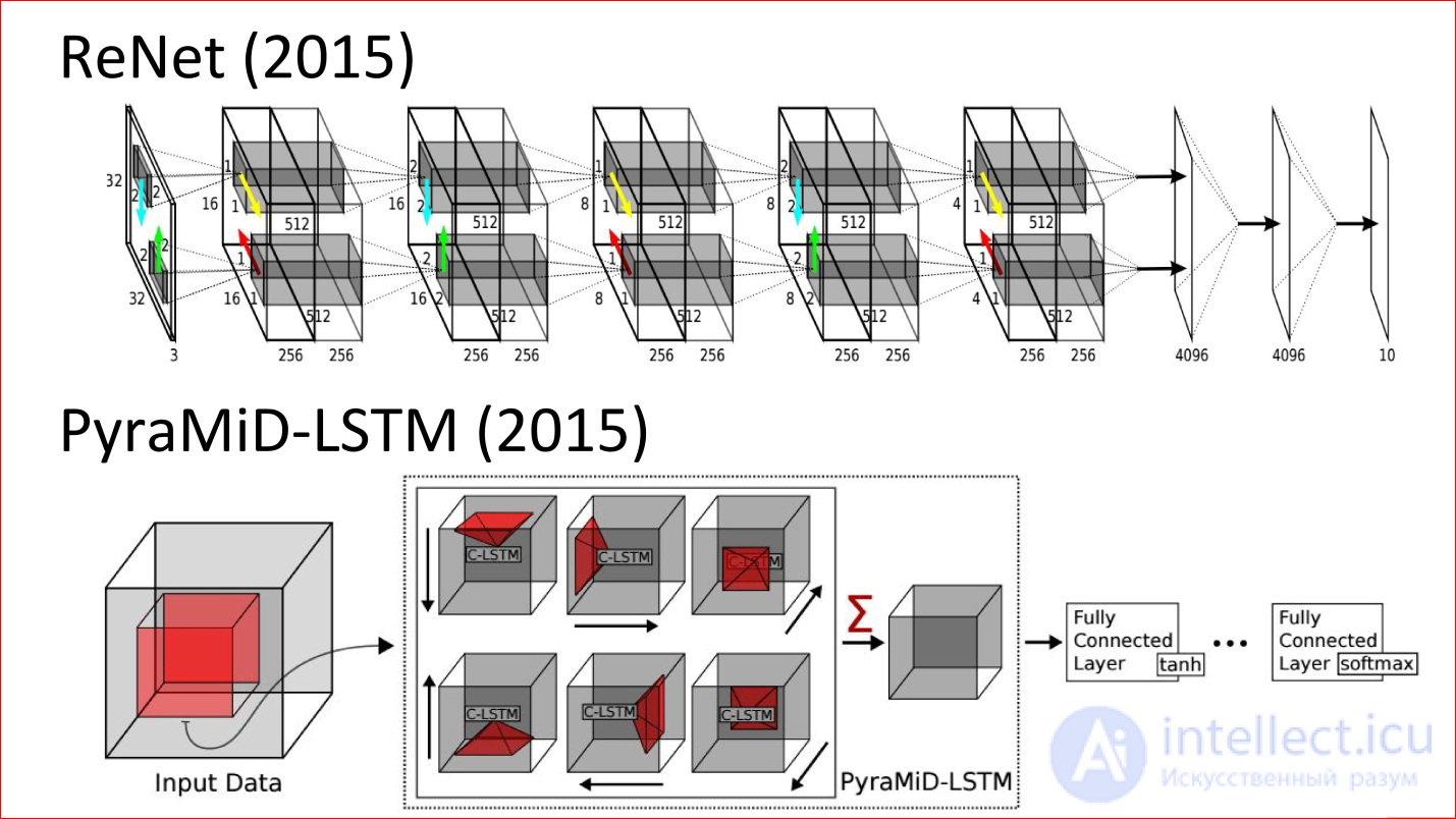
Here are the latest works (2015). This neural network is analogous to the classic LeNet neural network, which classified handwritten numbers. But now it is never convolutional, but recurrent and multidirectional. There are arrows that are in different directions in the image.
The second example is the tricky neural network, which was used for segmentation of brain sections. She, too, is never convolutional, but recurrent, and she won in some regular competition.
На самом деле это крутые технологии. Думаю, что в ближайшее время рекуррентные сети очень сильно потеснят сверточные потому, что даже для изображений они добавляют очень много чего. Это потенциально более мощный класс.
продолжение следует...
Часть 1 Introduction to neural network architectures. Classification of neural networks, principle of operation
Часть 2 Grigory Sapunov (Intento) - Introduction to neural network architectures. Classification
Часть 3 Мультимодальное обучение (Multimodal Learning) - Introduction to neural network architectures.

Comments
To leave a comment
Computational Neuroscience (Theory of Neuroscience) Theory and Applications of Artificial Neural Networks
Terms: Computational Neuroscience (Theory of Neuroscience) Theory and Applications of Artificial Neural Networks