Lecture
Vector space. Basis. Orthogonal projections. Hypersphere and hypersurfaces. Matrices. Linear transformations.
A mathematical language traditionally used to describe neural networks is the apparatus of vector and matrix algebra. For maximum simplification of presentation, limiting the set of general mathematical information only to this apparatus, I would like to emphasize that other branches of mathematics are widely used in modern neuroscience. Among them - the differential equations used to analyze neural networks in continuous time, as well as to build detailed models of the neuron; Fourier analysis to describe the behavior of the system when coding in the frequency domain; optimization theory as a basis for developing learning algorithms; mathematical logic and Boolean algebra - for describing binary networks, and others. The material presented in this lecture is for reference only and does not claim to be complete. Comprehensive information on the theory can be found in Gantmakher’s book, as well as in standard courses in linear algebra and analytic geometry.
The main structural element in the description of information processing methods by a neural network is a vector - an ordered set of numbers, called vector components . In the future, the vector will be denoted by Latin letters (a, b, c, x), and scalars - numbers - Greek letters ( a , b , g , q ). Matrix capital letters will be used to designate matrices. Depending on the characteristics of the problem under consideration, the vector components can be real numbers, whole numbers (for example, to denote image brightness gradations), as well as zero-one or minus one-one Boolean numbers. The components of the vector x = (x 1 , x 2 , ... x n ) can be considered as its coordinates in some n-dimensional space. In the case of real components, this space is denoted as R n and includes the set of all possible sets of n real numbers. The vector x is said to belong to the space R n (or x from R n ). In the future, if we need a set of vectors, we will be numbered by their superscripts, so as not to be confused with the numbering of the components: {x 1 , x 2 , ..., x k }.
In our consideration, we will not make a difference in terms of the vector (ordered set of components) and image (set of features or features of the image). Ways to select a set of features and the formation of the information vector are determined by specific applications.
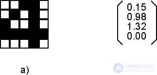
Fig. 2.1. Examples of vectors: a) a Boolean vector with 25 components, numbered in rows, b) a real vector from the space R 4 .
A set of vectors with real components is a special case of a more general concept, called a linear vector space V , if its elements are defined by the vector + and multiplication by scalar " . " Operations, which satisfy the following relations (here x, y, z are from V , a , b - scalars from R ):
Property 1) is called the co-mutability property, relations 2) and 3) are the distributivity property, and 4) the associativity property of the entered operations. An example of a linear vector space is the space R n with componentwise addition and multiplication.
For two elements of a vector space, their scalar (inner) product can be defined: (x, y) = x 1 y 1 + x 2 y 2 + ... + x n y n . Scalar product has the properties of symmetry, additivity and linearity for each factor:
The zero equality of the scalar product of two vectors means their mutual orthogonality, according to the usual geometric representations.
Two different images (or vectors) may be more or less similar to each other. For a mathematical description of the degree of similarity, the vector space can be equipped with a scalar metric - the distance d (x, y) between any two vectors x and y. Spaces with a given metric are called metric . For a metric, the conditions of non-negativity, symmetry, and the triangle inequality should be met:In the following, we will mainly use two metrics - the Euclidean distance and the Hamming metric . The Euclidean metric for a rectangular coordinate system is determined by the formula:

The Hamming distance d H is usually used for Boolean vectors (components of which are 0 or 1), and is equal to the number of components that are different in both vectors.
For vectors, the concept of the norm || x || - the length of the vector x. The space in which the norm of vectors is defined is called normalized . The norm should have the following properties:
Spaces with a Euclidean metric and norm are called Euclidean spaces. For images consisting of real signs, we will in the future deal specifically with Euclidean space. In the case of Boolean vectors of dimension n, the space under consideration is the set of vertices of the n-dimensional hypercube with the Hamming metric. The distance between two vertices is determined by the length of the shortest path connecting them, measured along the edges.
An important case for neural network applications is the set of vectors whose components are real numbers belonging to the [0,1] segment. The set of such vectors is not a linear vector space, since their sum may have components outside the considered segment. However, for a pair of such vectors, the concepts of the scalar product and the Euclidean distance are preserved.
The second interesting example, important from a practical point of view, is the set of vectors of the same length (equal, for example, to one). Figuratively speaking, the "tips" of these vectors belong to the hypersphere of unit radius in n-dimensional space. The hypersphere is also not a linear space (in particular, there is no zero element).
For a given set of features that define the space of vectors, such a minimal set of vectors can be formed, possessing these features to varying degrees, that on its basis, linearly combining vectors from the set, all possible other vectors can be formed. Such a set is called a space basis . Consider this important concept in more detail.
The vectors x 1 , x 2 , ..., x m are considered linearly independent if their arbitrary linear combination a 1 x 1 + a 2 x 2 + ... + a m x m does not vanish unless all the constants a 1 ... a m are not equal to zero at the same time. A basis can consist of any combination of n linearly independent vectors, where n is the dimension of space.
Choose a system of linearly independent vectors x 1 , x 2 , ..., x m , where m <n. All possible linear combinations of these vectors will form a linear space of dimension m, which will be a subspace or linear span of L of the original n-dimensional space. The chosen basic system of m vectors is obviously a basis in the subspace L. An important particular case of a linear hull is a subspace of dimension one less than the dimension of the original space (m = n-1), called the hyperplane . In the case of three-dimensional space, this is the usual plane. Hyperplane divides space into two parts. The set of hyperplanes breaks up the space into several sets, each of which contains vectors with a close set of features, thereby classifying the vectors.
For two subspaces, the concept of their mutual orthogonality can be introduced. Two subspaces L 1 and L 2 are said to be mutually orthogonal if every element of one subspace is orthogonal to each element of the second subspace.
Randomly selected linearly independent vectors are not necessarily mutually orthogonal. However, in some applications it is convenient to work with orthogonal systems. For this, the source vectors are required to be orthogonalized. The classical Gram-Schmidt orthogonalization process consists in the following: a system of orthogonal vectors h 1 , h 2 , ..., h m is recursively constructed using a system of linearly independent non-zero vectors x 1 , x 2 , ..., x m . As the first vector h 1 , the initial vector x 1 is chosen. Each next (i-th) vector is made orthogonal to all previous ones, for which its projections onto all previous vectors are subtracted from it:

Moreover, if any of the resulting vectors h i is equal to zero, it is discarded. It can be shown that, by construction, the resulting vector system turns out to be orthogonal, i.e. each vector contains only unique features.
Next will be presented the theoretical aspects of linear transformations on vectors.
Equal to the way the vector was considered - an object defined by a single index (the number of a component or feature), an object with two indices, a matrix , can also be entered. These two indices define the components of the matrix A ij , arranged in rows and columns, with the first index i specifying the row number, and the second j the column number. It is interesting to note that the image in Figure 2.1.a) can be interpreted both as a vector with 25 components, and as a matrix with five rows and five columns.
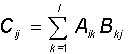
The sum of two matrices A and B of the same dimension (nxm) is the matrix C of the same dimension with components equal to the sum of the corresponding components of the original matrices: C ij = A ij + B ij . The matrix can be multiplied by a scalar, and the result is a matrix of the same dimension, each component of which is multiplied by this scalar. The product of two matrices A (nxl) and B (lxm) is also the matrix C (nxm), whose components are given by the relation:
Note that the dimensions of the matrices to be multiplied must be consistent — the number of columns of the first matrix must be equal to the number of rows of the second.
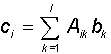
In the important particular case, when the second matrix is a vector (that is, a matrix with one of the dimensions equal to unity (m = 1)), the presented rule determines the method of multiplying the matrix by the vector:
As a result of multiplication, the vector c is also obtained, and for a square matrix A (lxl) its dimension is equal to the dimension of the factor vector b. With an arbitrary choice of the square matrix A, one can construct an arbitrary linear transformation y = T (x) of one vector (x) into another (y) of the same dimension: y = Ax. More precisely, in order for the transformation T of one vector to another to be linear, it is necessary and sufficient that for two vectors x 1 and x 2 and the numbers a and b , the equality holds: T ( a x 1 + b x 2 ) = a T (x 1 ) + b T (x 2 ). It can be shown that every linear transformation of vectors corresponds to multiplying the original vector by some matrix.
If in the above formula for multiplying the matrix A by the vector x, the components of this vector are unknown, while A and the resultant vector b are known, then the expression A x = b is referred to as a system of linear algebraic equations for the components of the vector x. The system has a unique solution if the vectors determined by the rows of the square matrix A are linearly independent.
Frequently used special cases of matrices are diagonal matrices in which all elements outside the main diagonal are zero. The diagonal matrix, all elements of the main diagonal of which are equal to one, is called the unit matrix I. The linear transformation defined by the unit matrix is the same: Ix = x for every vector x.
For matrices, besides the multiplication and addition operations, a transposition operation is also defined. The transposed matrix A T is obtained from the original matrix A by replacing the rows with columns: (A ij ) T = A ji . Matrices that do not change when transposed are called symmetric matrices . For the components of the symmetric matrix S, the relation S ij = S ji holds. Every diagonal matrix is obviously symmetric.
The space of square matrices of the same dimension with the introduced operations of addition and elementwise multiplication by a scalar is a linear space. For him, you can also enter the metric and norm. The zero element is the matrix, all elements of which are equal to zero.
In conclusion, we present some identities for operations on matrices. For all A, B and C and the identity matrix I takes place:

Comments
To leave a comment
Computational Neuroscience (Theory of Neuroscience) Theory and Applications of Artificial Neural Networks
Terms: Computational Neuroscience (Theory of Neuroscience) Theory and Applications of Artificial Neural Networks