6. Multi-layer PERSEPTRON.

Limitations of single-layer neural networks. The need for a hierarchical organization of the neural system. Multi-layer PERSEPTRON. Error Propagation Algorithm.

The need for a hierarchical organization of neural network architectures.

In previous lectures, we have already had to meet with very strict restrictions on the capabilities of single-layer networks, in particular, with the requirement of linear separability of classes. The structural features of biological networks push the investigator to use more complex, and in particular, hierarchical architectures. The idea is relatively simple - at lower levels of the hierarchy, classes are transformed in such a way as to form linearly separable sets, which in turn will be successfully recognized by neurons at the next ( higher ) levels of hierarchy.

However, the main problem traditionally limiting possible network topologies to the simplest structures is the problem of learning. At the network learning stage, some input images, called a training set, are revealed, and the resulting output reactions are investigated. The purpose of training is to bring the observed reactions on a given training set to the required (adequate) reactions by changing the states of synaptic connections. A network is considered trained if all reactions on a given set of incentives are adequate. This classical training scheme with the teacher requires an explicit knowledge of the errors in the functioning of each neuron, which, of course, is difficult for hierarchical systems, where only inputs and outputs are directly controlled. In addition, the necessary redundancy in hierarchical networks leads to the fact that the state of learning can be implemented in many ways, which makes the very concept of “error made by a given neuron” very uncertain.

The presence of such serious difficulties was largely hampered by the progress in the field of neural networks until the mid-80s, when effective algorithms for learning hierarchical networks were obtained.

Multi-layer PERSEPTRON.

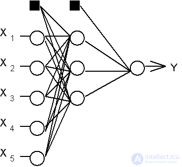
Consider a hierarchical network structure in which interconnected neurons (network nodes) are combined in several layers (Fig. 6.1). F. Rosenblatt pointed out the possibility of building such architectures, but he did not solve the problem of learning. The interneuron synaptic connections of the network are arranged in such a way that each neuron at a given level of the hierarchy receives and processes signals from each neuron of a lower level. Thus, in this network there is a dedicated direction of distribution of neuropulses - from the input layer through one (or several) hidden layers to the output layer of neurons. We will call a neural network of such a topology a generalized multilayer perceptron or, if it does not cause any misunderstanding, simply a perceptron.

Perceptron is a network consisting of several consecutively connected layers of McCulloch and Pitts formal neurons. At the lowest level of the hierarchy is the input layer, consisting of sensory elements, whose task is only to receive and distribute the input information through the network. Then there is one or, more rarely, several hidden layers. Each neuron on the hidden layer has several inputs connected to the outputs of the neurons of the previous layer or directly to the input sensors X 1..Xn, and one output. The neuron is characterized by a unique weight vector w. The weights of all the neurons in the layer form a matrix, which we will denote by V or W. The function of the neuron is to calculate the weighted sum of its inputs with further non-linear conversion into the output signal:

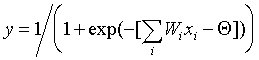(6.1)

The outputs of the neurons of the last, output layer describe the result of the classification Y = Y (X). Features of the perceptron work are as follows. Each neuron sums incoming signals from neurons of the previous level of the hierarchy with weights, determined by the states of synapses, and generates a response signal (goes into an excited state) if the resulting sum is above the threshold value. Perceptron translates the input image, which determines the degree of excitation of the neurons of the lowest level of the hierarchy, into the output image defined by the neurons of the highest level. The number of the latter is usually relatively small. The state of excitation of a neuron at the top level indicates that the input image belongs to one category or another.

Traditionally, analog logic is considered, in which the admissible states of synaptic connections are determined by arbitrary real numbers, and the degree of neuron activity is determined by real numbers between 0 and 1. Sometimes models with discrete arithmetic are also studied, in which the synapse is characterized by two Boolean variables: activity (0 or 1) and polarity (-1 or +1), which corresponds to the three-valued logic. The states of the neurons can then be described by a single Boolean variable. This discrete approach makes the configuration space of the states of the neural network finite (not to mention the advantages of the hardware implementation).

Here, the classic version of a multilayered network with analog synapses and a sigmoidal neuron transfer function defined by formula (6.1) will be described here.

Training method back propagation of errors.

For teaching a multilayer network in 1986, Rummelhart and Hinton (Rummelhart DE, Hinton GE, Williams RJ, 1986) proposed an error back propagation algorithm. Numerous publications on industrial applications of multilayer networks with this learning algorithm have confirmed its principal performance in practice.

At the outset, a reasonable question arises - why can't the already well-known d- rule of Rosenblatt (see Lecture 4) not be used for teaching a multilayer perceptron? The answer is that to apply the Rosenblatt method, it is necessary to know not only the current outputs of the neurons y, but also the required correct values ​​of Y. In the case of a multilayer network, these correct values ​​are available only for neurons of the output layer. The required output values ​​for neurons of hidden layers are unknown, which limits the use of the d- rule.

The basic idea of ​​backpropagation is how to get an error estimate for neurons of hidden layers. Note that the known errors made by the neurons of the output layer arise due to the so far unknown errors of the neurons of the hidden layers. The greater the value of the synaptic connection between the neuron of the hidden layer and the output neuron, the stronger the error of the first affects the error of the second. Therefore, the error estimate of the elements of hidden layers can be obtained as a weighted sum of the errors of the subsequent layers. When training, information is distributed from the lower layers of the hierarchy to the highest, and the error estimates made by the network are reversed, which is reflected in the name of the method.

Let us turn to a detailed review of this algorithm. To simplify the notation, we limit ourselves to the situation when the network has only one hidden layer. The matrix of weights from the inputs to the hidden layer is denoted by W, and the matrix of weights connecting the hidden and output layers - as V. For indexes, we take the following notation: the inputs will be numbered only by index i, the elements of hidden layer - by index j, and the outputs, respectively, by index k.

Let the network be trained on the sample (X a , Y a ), a = 1..p. The activity of neurons will be denoted by small letters y with the corresponding index, and the total weighted inputs of neurons by small letters x.

The general structure of the algorithm is similar to that discussed in Lecture 4, with the complication of the weight adjustment formulas.

Table 6.1. Error propagation algorithm.

Step 0.	The initial values ​​of the weights of all neurons of all layers of V (t = 0) and W (t = 0) are assumed to be random numbers.
Step 1.	The input image X a is presented to the network, and as a result, the output image y ¹ Y a is formed . At the same time, neurons sequentially from layer to layer function according to the following formulas: hidden layer 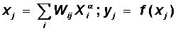output layer Here f (x) is a sigmoidal function defined by the formula (6.1)
Step 2.	The functional of the quadratic network error for a given input image is: 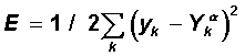This functionality is subject to minimization. The classical gradient optimization method consists in iterative refinement of the argument according to the formula: 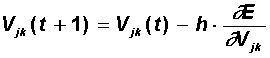The error function does not explicitly contain a dependence on the weight V jk , so we use the implicit differentiation formulas for a complex function: 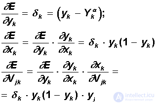Here, the useful property of the sigmoidal function f (x) is taken into account: its derivative is expressed only through the value of the function itself, f '(x) = f (1-f). Thus, all the necessary values ​​for adjusting the weights of the output layer V are obtained.
Step 3.	At this step, the adjustment of the scales of the hidden layer is performed. The gradient method still gives: 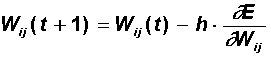Calculations of derivatives are performed using the same formulas, with the exception of some complication of the formula for the error d j . When calculating d j here, the principle of back propagation of error was applied: partial derivatives are taken only on variables of the next layer. According to the obtained formulas, the weights of the neurons of the hidden layer are modified. If there are several hidden layers in the neural network, the back-propagation procedure is applied sequentially for each of them, starting with the layer preceding the output layer and then to the layer following the input one. In this case, the formulas retain their appearance with the replacement of the elements of the output layer by the elements of the corresponding hidden layer.
Step 4.	Steps 1-3 are repeated for all training vectors. Training ends when a small total error is reached or the maximum number of iterations is reached, as in the Rosenblatt teaching method.

As can be seen from the description of steps 2-3, learning is reduced to solving the problem of optimizing the error functional by the gradient method. The whole “salt” of the back propagation of an error consists in the fact that for its evaluation for neurons of hidden layers one can accept a weighted sum of errors of the next layer.

The parameter h has the meaning of the learning rate and is chosen small enough for the method to converge. On convergence, you need to make a few additional observations. First, practice shows that the convergence of the back propagation method is very slow. The low heat of convergence is a “genetic disease” of all gradient methods, since the local direction of the gradient does not coincide with the direction to the minimum. Secondly, the adjustment of the weights is performed independently for each pair of images of the training sample. At the same time, an improvement in the functioning on a certain given pair can, generally speaking, lead to a deterioration in the operation on previous images. In this sense, there are no reliable (except for the very extensive practice of applying the method) guarantees of convergence.

Studies show that in order to represent an arbitrary functional mapping defined by a training set, only two layers of neurons are sufficient. However, in practice, in the case of complex functions, the use of more than one hidden layer can save the total number of neurons.

At the end of the lecture, we make a remark regarding the setting of the thresholds of neurons. It is easy to see that the neuron threshold can be made equivalent to the additional weight connected to the dummy input, equal to -1. Indeed, choosing W ₀ = Q , x ₀ = -1 and starting from zero summation, we can consider a neuron with a zero threshold and one additional input:

The additional inputs of the neurons corresponding to the thresholds are shown in Fig. 6.1 dark squares. Taking this remark into account, all the summation formulas for inputs stated in the back-propagation algorithm begin with a zero index.