8. Hopfield model

Configuration and stability of networks with feedback. Hopfield model. The rule of learning Hebba. Associative memory. Pattern recognition.

The Hopfield model (JJHopfield, 1982) occupies a special place among the neural network models. It was the first to succeed in establishing a connection between nonlinear dynamical systems and neural networks. The images of the network memory correspond to the stable limit points (attractors) of the dynamical system. The possibility of transferring the mathematical apparatus of the theory of nonlinear dynamic systems (and statistical physics in general) to neural networks turned out to be especially important. At the same time, it became possible to theoretically estimate the memory volume of the Hopfield network, to determine the area of ​​network parameters in which the best functioning is achieved.

In this lecture, we will sequentially begin with the general properties of networks with feedback, establish a learning rule for the Hopfield network (Hebb's rule), and then proceed to discuss the associative memory properties of this neural network when solving the pattern recognition problem.

Networks with feedback

The PERSEPTRON considered by us earlier belongs to the class of networks with a directional flow of information distribution and does not contain feedback. At the stage of operation, each neuron performs its function - the transfer of excitation to other neurons - exactly once. The dynamics of neuron states is non-iterative.

Somewhat more complex is the dynamics in the Kohonen network. Competition of neurons is achieved by iterations, in the process of which information is repeatedly transmitted between neurons.

In the general case, a neural network (see Fig. 8.1) can be considered, containing arbitrary feedbacks , through which the transmitted excitation returns to the neuron, and it re-performs its function. Observations on biological local neural networks indicate the presence of multiple feedbacks. Neurodynamics in such systems becomes iterative. This property significantly expands many types of neural network architectures, but at the same time leads to the emergence of new problems.

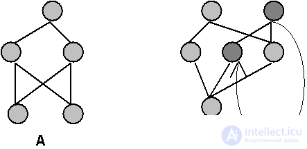
The non-iterative dynamics of the states of neurons is obviously always stable. Feedbacks can lead to instabilities , like those that occur in amplifying radio-technical systems with positive feedback. In neural networks, the instability manifests itself in a wandering change in the states of neurons, which does not lead to the appearance of stationary states. In the general case, the answer to the question of the stability of the dynamics of an arbitrary system with feedbacks is extremely complicated and is still open.

Below we dwell on the important particular case of the neural network architecture, for which the properties of stability are studied in detail.

Neurodynamics in the Hopfield model

Consider a network of N formal neurons in which the degree of excitation of each of the neurons S _i , i = 1..N, can take only two values ​​{-1, +1}. Any neuron has a connection with all other neurons S _j , which in turn are connected with it. The connection strength from the i-th to the j-th neuron is denoted as W _ij .

The Hopfield model assumes the condition of symmetry of the bonds W _ij = W _ji , with zero diagonal elements W _ii = 0. Unfortunately, this condition is very remotely related to the known properties of biological networks, in which, on the contrary, if one neuron transmits excitation to another, then it, in most cases, is not directly connected with the first one. However, it is the symmetry of the bonds, as will be clear from what follows, that significantly affects the stability of the dynamics.

The change in the state of each neuron S _j in the Hopfield model occurs according to the well-known rule for formal neurons of McCullock and Pitts. The signals S _i arriving at its inputs at time t are weighted with the weights of the matrix of relations W _ij and summed up, determining the total level of the input signal strength:

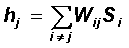
Then at the time t + 1, a neuron changes its state of excitation depending on the signal level h and the individual threshold of each neuron T:

A change in the excitation states of all neurons can occur simultaneously, in which case they are talking about parallel dynamics. Sequential neurodynamics is also considered, in which at a given moment in time there is a change in the state of only one neuron. Numerous studies have shown that the memory properties of a neural network are practically independent of the type of dynamics. When simulating a neural network on a regular computer, it is more convenient to successively change the states of the neurons. In hardware implementations of Hopfield neural networks, parallel dynamics will be applied.

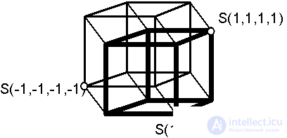
The set of values ​​of excitation of all neurons S _i at some moment of time forms the state vector S of the network. Neurodynamics leads to a change in the state vector S (t). The state vector describes the trajectory in the state space of the neural network. This space for a network with two levels of excitation of each neuron is obviously a set of vertices of a hypercube of dimension equal to the number of neurons N. Possible sets of coordinate values ​​of the vertices of the hypercube (see Fig. 8.2) and determine the possible values ​​of the state vector.

We now consider the problem of the stability of the dynamics of state change. Since at each time step a certain neuron i changes its state in accordance with the sign of the magnitude (h _i - T _i ), the relationship below is always non-positive:

Thus, the corresponding value of E, which is the sum of the individual values ​​of E _i , can only decrease or retain its value in the process of neurodynamics.

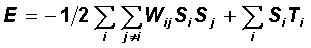
The value E introduced in this way is a function of the state E = E ( S ) and is called the energy function (energy) of the Hopfield neural network. Since it has the property of non-increasing with network dynamics, at the same time it is a Lyapunov function for it (AM Lyapunov, 1892). The behavior of such a dynamic system is stable for any initial state vector S (t = 0) and for any symmetric matrix of relations W with zero diagonal elements. In this case, the dynamics ends in one of the minima of the Lyapunov function, and the activity of all neurons will coincide in sign with the input signals h.

The energy surface E ( S ) in the state space has a very complex shape with a large number of local minima, vividly resembling a quilt. Stationary states corresponding to minima can be interpreted as images of the neural network memory. Evolution to this image corresponds to the process of extracting from memory. For an arbitrary connection matrix W, the images are also arbitrary. To write any meaningful information to the network memory, a certain value of weights W is needed, which can be obtained in the learning process.

Hebb's learning rule

The learning rule for the Hopfield network is based on research by Donald Hebb (D.Hebb, 1949), who suggested that the synaptic connection connecting the two neurons will be enhanced if both neurons in the process of learning are consistently excited or inhibited. A simple algorithm that implements such a learning mechanism is called the Hebbian rule . Consider it in detail.

Let the training sample of images x _a , a = 1..p be given. It is required to construct the process of obtaining the matrix of connections W, such that the corresponding neural network will have the images of the training sample as stationary states (the values ​​of the thresholds of neurons T are usually set equal to zero).

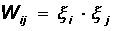
In the case of a single training image, Hebb's rule leads to the required matrix:

Let us show that the state S = x is stationary for the Hopfield network with the indicated matrix. Indeed, for any pair of neurons i and j, the energy of their interaction in the state x reaches its minimum possible value E _ij = - (1/2) x _i x x x _i x _j = -1/2.

In this case, E is the total energy equal to E = - (1/2) N ² , which corresponds to the global minimum.

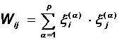
An iterative process can be used to memorize other images:

which leads to a complete matrix of connections in the form of Hebb:

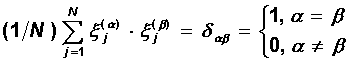
The stability of the totality of images is not as obvious as in the case of a single image. A number of studies show that a neural network trained according to Hebb's rule can, on average, with a large network size N, store no more than p » 0.14 N different images. Resilience can be shown for a collection of orthogonal patterns when

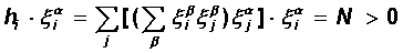
In this case, for each state x ^{a, the} product of the total input of the i-th neuron h _i by the amount of its activity S _i = x ^a _i turns out to be positive, therefore the state x a itself is a state of attraction (stable attractor ):

Thus, the Hebba rule ensures the stability of the Hopfield network on a given set of relatively few orthogonal patterns. In the next paragraph, we will focus on the memory features of the resulting neural network.

Memory associativity and pattern recognition task

The dynamic process of successive change of states of the Hopfield neural network ends in a certain stationary state, which is the local minimum of the energy function E ( S ). The non-growth of energy in the course of dynamics leads to the choice of such a local minimum S , in the basin of attraction of which the initial state (the initial image predicted by the network) S ₀ falls. In this case, it is also said that the state S ₀ is in the bowl of the minimum S.

With sequential dynamics, an image S will be chosen as the stationary state, which will require the minimum number of state changes of individual neurons. Since for two binary vectors the minimum number of component changes that translates one vector into another is the Hamming distance r _H ( S, S ₀ ), it can be concluded that the network dynamics ends at the local minimum of energy closest to the Hamming.

Let state S correspond to some ideal memory image. Then the evolution from state S ₀ to state S can be compared with the procedure of gradual restoration of an ideal image S from its distorted (noisy or incomplete) copy S ₀ . Memory with such properties of the process of reading information is associative . When searching, the distorted parts of the whole are restored to the existing undistorted parts based on the associative links between them.

The associative nature of the Hopfield network memory qualitatively distinguishes it from ordinary, address, computer memory. In the latter, the extraction of the necessary information occurs at the address of its starting point (memory cell). The loss of the address (or even the address bit of the address) results in the loss of access to the entire information fragment. When using associative memory, access to information is made directly according to its content , i.e. by partially known distorted fragments. The loss of a part of information or its informational noise does not lead to a catastrophic access restriction, if the remaining information is enough to extract the ideal image.

The search for the ideal image from the existing incomplete or noisy version of it is called the pattern recognition task. In our lecture, the features of the solution of this problem by the Hopfield neural network will be demonstrated by examples obtained using the network model on a personal computer.

In the model under consideration, the network contained 100 neurons arranged in a 10 x 10 matrix. The network was trained according to Hebb's rule in three ideal images - the font styles of the Latin letters M, A and G (Fig. 8.3.). After learning of the neural network, various distorted versions of the images were presented as the initial states of the neurons, which later evolved with consistent dynamics to stationary states.

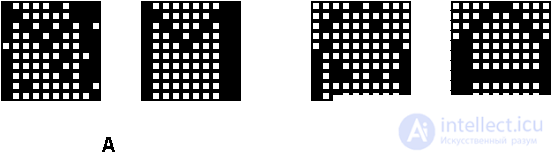
For each pair of images in the pictures on this page, the left image is the initial state, and the right image is the result of the network operation, the stationary state reached.

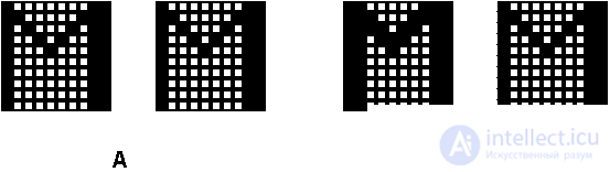
The image in Fig. 8.4. (A) was chosen to test the adequacy of behavior on an ideal task, when the displayed image exactly matches the information in memory. In this case, a steady state was achieved in one step. The image in Fig. 8.4. (B) is characteristic for text recognition tasks, regardless of the type of font. The initial and final images are certainly similar, but try to explain this to the machine!

Tasks in Fig. 8.5 are typical for practical applications. The neural network system is able to recognize almost completely noisy images. Tasks corresponding to Pic. 8.6. and 8.7. (B) demonstrate the remarkable property of the Hopfield network to associatively recognize an image by its small fragment. The most important feature of the network is the generation of false images. An example of relaxation to a false image is shown in Fig. 8.7. (A). A false image is a stable local extremum of energy, but does not correspond to any ideal image. He is in a sense a collective way, inheriting the features of ideal brethren. The situation with a false image is equivalent to our "Somewhere I have already seen it."

In this simplest task, a false image is a “wrong” solution, and therefore harmful. However, one can hope that such a tendency of the network to generalize can certainly be used. It is characteristic that with an increase in the volume of useful information (compare Fig. 8.7. (A) and (B)), the initial state falls into the region of attraction of the desired stationary state, and the image is recognized.

Despite the interesting qualities, the neural network in the classical Hopfield model is far from perfect. It has a relatively modest memory size proportional to the number of neurons in the network N, while address memory systems can store up to 2N different images using N bits. In addition, Hopfield neural networks cannot solve the recognition problem if the image is displaced or rotated relative to its original stored state. These and other shortcomings today define a general attitude towards the Hopfield model, rather as a theoretical structure, convenient for research, than as a daily practical tool.

In the following lectures, we will look at the development of the Hopfield model, modifications of the Hebbian rule, which increase the memory space, as well as the application of probability generalizations of the Hopfield model to combinatorial optimization problems.