Lecture
Let's make the simplest mathematical model of the process of evolution. Consider systems in which the change in time of a certain parameter  =
=  proportional to the value of this parameter, i.e. ~ q. Such systems are called autocatalytic. The parameter q may include concentration, temperature, the number of people on the planet, etc. The simplest evolutionary equation takes the form
=  q,
q,
- a parameter that determines both the speed and the nature of the process change.
The solution to this equation is:
q = q 0 e  ,
,
at the initial moment of time  = 0
= 0
Parameter may be a positive, negative, imaginary quantity, which determines the nature of evolution. For example, when > 0 the process goes in the direction of increasing q according to the law of the exponent, with <0 - according to the law of decreasing exponentially, with = i a - the process obeys the harmonic law, and for the complex value of the parameter = b + i and an evolution occurs with a combination of exponential and complex laws (Fig. 1).
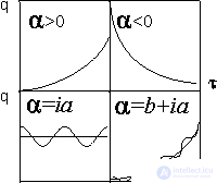
Figure 1. The dependence of the parameter q on for different types .
As previously indicated, synergistic systems are characterized by stochasticity, i.e. their time dependence cannot be predicted with absolute accuracy. Therefore, for such systems, the term f ( ), taking into account fluctuations in the system, i.e.
= q + f ( ).
Consider a more complicated case: substance 1 with a concentration of q 1 is formed autocatalytically ( ~ q) as a result of interaction with substance 2, the concentration of which is q 2 , then

 - proportionality coefficient, having the same meaning as the parameter .
Given the stochasticity of the synergistic system, the evolution equation will take the form
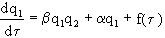 .
.
With the help of the last equation it is possible to describe various types of population behavior. In this equation, b describes the nature of the relationship between the parameters q 1 and q 2 and, if it is regulated externally, then b plays the role of a control parameter.
In real synergistic systems there are a lot of subsystems q 1 , q 2 , ..., q n , and when compiling a mathematical model, it is important to distinguish levels of description: microscopic (atoms, molecules), mesoscopic (ensemble of atoms and molecules), macroscopic (extended regions and molecules and their ensembles). For example, when describing crystal growth, evolutionary equations contain the parameters q 1 (x, ) - the density of the substance in the liquid and q 2 (x, ) - in the solid phase. From the equations it is possible to determine the formation in time of the solid phase q 2 ( ) depending on the density in the liquid phase q 1 (x, ), i.e. q 2 ( ) = f (q 1 , ).
Population size . We first consider the dynamics of populations, that is, what factors control the number of populations, how many different populations can coexist. Let's start with any one population (bacteria, plants, animals of this species). The main characteristic is the number of individuals n in the population. It varies with the rate of birth (number of births) g and the speed of death (number of deaths) d:
 = gd
= gd
Birth and death rates depend on the number of individuals available.
g =  n, d =
  n,
n,
where are the coefficients and do not depend on n, i.e. growth does not depend on population density. But they depend on such parameters as the amount of available food, temperature, climate, etc. With a constant value of these factors
= n = ( - )
This equation describes either an exponentially growing or an exponentially decreasing population, but a steady state = 0 is impossible, and for the existence of a process it should be assumed that the coefficients and must depend on density. The reason for the latter is also associated with restrictions in food. If we consider the depletion of power sources, then, as shown above, we turn to the Verhulst equation
= 0 - n 2
This equation has significant self-worth, so we strongly recommend ALL to read the paragraph devoted to it.
Models of competition and coexistence . If different species do not eat the same food and do not interact with each other, they can coexist. The equations for the number of species j are written as
j = j - j n j 2 , j = 1, 2, ...
The situation is complicated if different species live off of the same food source, and they depend on the same living conditions.
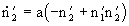
Let n 1 and n 2 be the numbers of individuals of two species that feed from the same food source N 0 . Under this condition, only one species survives, and the other dies out, since the species with a larger breeding constant eats food much faster than other species. It should be noted that the amount of food is not set at the initial moment, but comes constantly with a certain speed.
For a population to survive, it is important to improve its individual constants. j and j by adapting, and also important is the additional intake of food. Consider two types 1 and 2, living at the expense of "overlapping" power sources. This situation can be simulated by the equations
= ( 11 N 1 + 12 N 2 ) * n 1 - 1 n 1
= ( 21 N 1 + 22 N 2 ) * n 2 - 2 n 2
Model predator - the victim. This model is in the literature the name of the model Lotka-Voltaire. Consider the existence in the sea of two types of fish - predator fish and prey fish. The rate of change of populations j = 1, 2 is given by the equation
1 = Increment j - Loss j , j = 1, 2.
Denote the victim fish by index 1. If there are no predators, the victim fish will multiply according to the law.
Gain 1 = 1 n 1 .
But prey fish are eaten by predators and the number of prey fish decreases, and the losses are proportional to the number of prey n 1 and predator n 2
Loss 1 = n 1 n 2 .
We now consider the equation for j = 2 (predator fish). Since predators live off of prey, the rate of predator reproduction is proportional to their own number and the number of prey.
Increment 2 = n 1 n 2 ,
Losses 2 = 2  2 n 2 .
So, the equations of the Lotka-Voltaire model are
= 1 n 1 + n 1 n 2
= n 1 n 2 - 2 2 n 2
These equations can be reduced to a dimensionless form.
 ,
,
 ,
,
If we put
 ,
,  ,
,  .
.
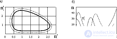
Figure 2. Two typical trajectories on the plane (n 1 ', n 2 ') in the Lotka-Voltaire model (f),
time variation of the populations n 1 'and n 2 ' (b).
In fig. 2a shows two typical trajectories on the plane (n 1 ', n 2 ') in the Lotka-Voltaire model with fixed parameters. It follows from this figure that the change in n 1 and n 2 is periodic (Fig. 2b): when predators reproduce too strongly, then the victims are destroyed by them very quickly. Therefore, food stocks in predators are reduced and the number of predators decreases accordingly. As a result, the number of animal victims increases, i.e., the food stocks of predators are growing, which are beginning to reproduce again.

Comments
To leave a comment
Synergetics
Terms: Synergetics