Lecture
The word “statistics” is often associated with the word “mathematics”, and it frightens students who associate this concept with complex formulas that require a high level of abstraction.
However, as McConnell says, statistics is primarily a way of thinking, and to apply it you just need to have some common sense and know the basics of mathematics. In our daily life, we ourselves, without realizing it, are constantly engaged in statistics. Do we want to plan a budget, calculate the gasoline consumption of a car, estimate the efforts required to master a certain course, taking into account the marks obtained so far, consider the probability of good and bad weather according to the meteorological report, or even estimate the impact of this or that event on our personal or joint future - we constantly have to select, classify and organize information, link it with other data so that we can draw conclusions that allow us to make the right decision.
All these types of activities differ little from those operations that underlie scientific research and consist in synthesizing data obtained from different groups of objects in a given experiment, in their comparison with the aim of finding out the features of the differences between them, in comparing them in order to identify indicators, changing in one direction, and, finally, in predicting certain facts on the basis of the conclusions to which the obtained results lead. This is precisely the purpose of statistics in the sciences in general, especially in the humanities. In the latter, there is nothing absolutely reliable, and without statistics, the conclusions in most cases would be purely intuitive and could not form a solid basis for interpreting data obtained in other studies.
In order to appreciate the enormous benefits that statistics can provide, we will try to follow the process of decoding and processing the data obtained in the experiment. Thus, on the basis of specific results and the questions that they pose to the researcher, we will be able to understand the various techniques and simple ways to apply them. However, before embarking on this work, it will be useful for us to consider in the most general terms the three main sections of statistics.
1. Descriptive statistics , as the name suggests, allows you to describe, summarize and reproduce in the form of tables or graphs
data of a particular distribution , calculate the average for a given distribution and its scope and variance .
2. The task of inductive statistics is to check whether the results obtained on this sample can be extended to the entire population from which this sample is taken. In other words, the rules of this section of statistics allow us to find out to what extent it is possible, by induction, to generalize to a greater number of objects one or another regularity found in the study of their limited group in the course of an observation or experiment. Thus, with the help of inductive statistics, some conclusions and generalizations are made, based on the data obtained from the study of the sample.
3. Finally, measuring the correlation lets you know how closely the two variables are related, so that you can predict the possible values of one of them, if we know the other.
There are two types of statistical methods or tests that allow generalizing or calculating the degree of correlation. The first type is the most widely used parametric methods , in which parameters such as mean value or data variance are used. The second type is non-parametric methods that provide an invaluable service in the case when the researcher deals with very small samples or qualitative data; These methods are very simple in terms of both calculations and applications. When we get acquainted with the various ways of describing data and move on to their statistical analysis, we consider both of these varieties.
As already mentioned, in order to try to understand these different areas of statistics, we will try to answer the questions that arise in connection with the results of a particular study. As an example, we take one experiment, namely, the study of the effect of marijuana consumption on the oculomotor coordination and on the reaction time. The methodology used in this hypothetical experiment, as well as the results that we could get in it, are presented below.
If you wish, you can replace some specific details of this experiment with others - for example, marijuana consumption with alcohol consumption or sleep deprivation - or, even better, substitute those hypothetical data for those that you actually received in your own research. In any case, you will have to accept the “rules of our game” and perform the calculations that are required of you here; only under this condition will the creature of the object “reach” you, if this has not happened to you before.
Important note. In the sections devoted to descriptive and inductive statistics, we will consider only those experimental data that are related to the dependent variable "hit targets". As for such an indicator as the reaction time, we turn to it only in the section on calculating the correlation. However, it goes without saying that from the very beginning, the values of this indicator should be processed in the same way as the variable “hit targets”. We provide the reader to do this on their own with pencil and paper.
One of the tasks of statistics is to analyze the data obtained on the part of the population in order to draw conclusions regarding the population as a whole.
A population in statistics does not necessarily mean a group of people or a natural community; this term refers to all beings or objects that make up the common population studied, whether they are atoms or students visiting a particular cafe.
The sample is a small number of elements selected using scientific methods so that it is representative, i.e. reflected the population as a whole.
(In the domestic literature, the terms “general set” and “selective set”, respectively, are more common. - Approx. Transl. )
Data in statistics are the main elements to be analyzed. Data may be some quantitative results, properties inherent in certain members of the population, a place in one sequence or another - in general, any information that can be classified or categorized for processing.
Do not mix “data” with those “values” that this data can accept. In order to always distinguish between them, Chatillon (Chatillon, 1977) recommends memorizing the following phrase: “Data often takes the same values” (so if we take, for example, six data - 8, 13, 10, 8, 10 and 5, they take only four different values - 5, 8, 10 and 13).
Distribution construction is the division of primary data obtained in a sample into classes or categories in order to obtain a generalized, ordered picture that allows them to be analyzed.
There are three types of data:
1. Quantitative data obtained during measurements (for example, data on weight, dimensions, temperature, time, test results, etc.). They can be distributed on a scale with equal intervals.
2. Ordinal data corresponding to the places of these elements in the sequence obtained when they are arranged in ascending order (1st, ..., 7th, ..., 100th, ...; A, B, B. ...).
3. Qualitative data representing some properties of the elements of the sample or population. They cannot be measured, and their only quantitative estimate is the frequency of occurrence (the number of people with blue or green eyes, smokers and non-smokers, tired and rested, strong and weak, etc.).
Of all these types of data, only quantitative data can be analyzed using methods based on parameters (such as, for example, arithmetic mean). But even to quantitative data such methods can be applied only if the number of these data is sufficient for the normal distribution to manifest. So, for the use of parametric methods, in principle, three conditions are necessary: the data should be quantitative, their number should be sufficient, and their distribution should be normal. In all other cases, it is always recommended to use non-parametric methods.
Descriptive statistics allows you to summarize the primary results obtained from observation or experiment. The procedures here are reduced to grouping data by their values, building the distribution of their frequencies, identifying the central distribution trends (for example, the arithmetic mean) and, finally, to estimating the spread of data with respect to the found central trend.
Hypothetical experiment. The effect of marijuana consumption on oculomotor coordination and reaction time
A group of 30 student volunteers and female students who smoke regular cigarettes, but not marijuana, was conducted an experiment to study oculomotor coordination. The task of the test subjects was to hit moving targets shown on the display by manipulating the moving lever. Each subject was presented with 10 sequences of 25 targets.
In order to establish the initial level, we calculated the average number of hits from 25, as well as the average response time for 250 attempts. Then the group was divided into two subgroups as equally as possible. Seven girls and eight boys from the control group got a cigarette with regular tobacco and dried grass, the smoke from which reminded of the smoke of marijuana. In contrast, seven girls and eight boys from the experimental (experimental) group received a cigarette with tobacco and marijuana. Having smoked a cigarette, each test subject was again tested on. oculomotor coordination.
In tab. Figures 1 and 2 show the average results of both measurements for the subjects of both groups before and after exposure.
Table 1. The effectiveness of the subjects of the control and experimental groups (the average number of hit targets out of 25 in 10 test series)
| Control group | Experienced group | ||||
| Test subjects | Background (follow-up) | After exposure (tobacco with a neutral additive) | Test subjects | Background (before exposure) | After exposure (tobacco with marijuana) |
| D1 | nineteen | 21 | D8 | 12 | eight |
| 2 | ten | eight | 9 | 21 | 20 |
| 3 | 12 | 13 | ten | ten | 6 |
| four | 13 | eleven | eleven | 15 | eight |
| five | 17 | 20 | 12 | 15 | 17 |
| 6 | 14 | 12 | 13 | nineteen | ten |
| 7 | 17 | 15 | 14 | 17 | ten |
| Y1 | 15 | 17 | U9 | 14 | 9 |
| 2 | 14 | 15 | ten | 13 | 7 |
| 3 | 15 | 15 | eleven | AND | eight |
| four | 17 | 18 | 12 | 20 | 14 |
| five | 15 | sixteen | 13 | 15 | 13 |
| 6 | 18 | 15 | 14 | 15 | sixteen |
| 7 | nineteen | nineteen | 15 | 14 | eleven |
| eight | 22 | 25 | sixteen | 17 | 12 |
| Total | 237 | 240 | Total | 228 | 169 |
| Average | 15.8 | 16,0 | Average | 15.2 | 11.3 |
| Standard deviation | 3.07 | 4.25 | Standard deviation | 3.17 | 4.04 |
| Girls: D1-D14 | Boys: U1-U16 | ||||
Table 2. Reaction time of the subjects of the control and experimental groups (average time is 1/10 s in a series of 10 tests)
| Control group | Experienced group | ||||
| Test subjects | Background (before exposure) | After exposure (tobacco with a neutral additive) | Test subjects | Background (before exposure) | After exposure (tobacco with marijuana) |
| D 1 | eight | 9 | D 8 | 15 | 17 |
| 2 | 15 | sixteen | 9 | eleven | 13 |
| 3 | 13 | 14 | ten | sixteen | 20 |
| four | 14 | 13 | eleven | 13 | 18 |
| five | 15 | 12 | 12 | 18 | 21 |
| 6 | 13 | 15 | 13 | 14 | 22 |
| 7 | 14 | 15 | 14 | 13 | nineteen |
| Y1 | 12 | ten | U9 | 15 | 20 |
| 2 | sixteen | 13 | ten | 18 | 17 |
| 3 | 13 | 15 | eleven | 15 | nineteen |
| four | eleven | 12 | 12 | eleven | 14 |
| five | 18 | 13 | 13 | 14 | 12 |
| 6 | 12 | AND | 14 | eleven | 18 |
| 7 | 13 | 12 | 15 | 12 | 21 |
| eight | 14 | ten | sixteen | 15 | 17 |
| Average | 13.4 | 12.7 | Average | 14.06 | 17.9 |
| Standard deviation | 2.29- | 2.09 | Standard deviation | 2.28 | 2.97 |
| Girls: D1-D14 | Boys: U1-U16 | ||||
Data grouping
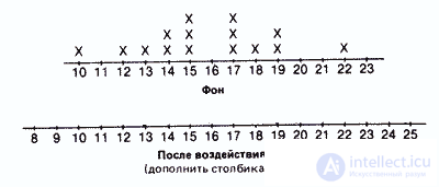
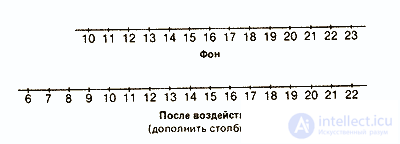
For grouping it is necessary first of all to arrange the data of each sample in ascending order. So, in our experiment for the variable "number of targets hit" the data will be located as follows:
Control group
| Background: | ten | 12 | 13 | 14 | 14 | 15 | 15 | 15 | 17 | 17 | 17 | 18 | nineteen | nineteen | 22 |
| After exposure: | eight | eleven | 12 | 13 | 15 | 15 | 15 | 15 | sixteen | 17 | 18 | nineteen | 20 | 21 | 25 |
Experienced group (add numbers yourself)
Background: ............
After exposure: .......
Frequency distribution (number of targets hit)
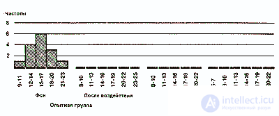
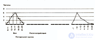
Already at the first glance, not obtained rows can be noticed that many data take the same values, and some values are more common and others less often. Therefore, it would be interesting to first graphically present the distribution of various values with regard to their frequencies. At the same time receive the following bar charts:
Control group
Experienced group
This distribution of data according to their values gives us much more than a representation in the form of rows. However, this grouping is used mainly only for qualitative data, clearly divided into separate categories.
As for quantitative data, they are always located on a continuous scale and, as a rule, are quite numerous. Therefore, such data is preferred to be grouped into classes, so that the main trend of distribution is more clearly visible.
Such a grouping consists mainly of combining data with the same or similar values into classes and determining the frequency for each class. The method of splitting into classes depends on what exactly the experimenter wants to reveal when dividing the measuring scale into equal intervals. For example, in our case, you can group the data into classes with intervals of two or three scale units:
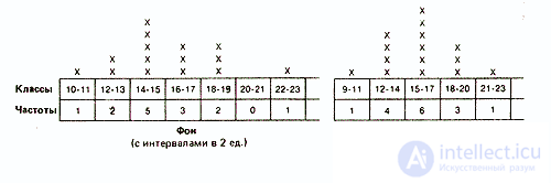

The choice of one or another type of grouping depends on various considerations. So, in our case, grouping with intervals between classes of two units well reveals the distribution of results around the central “peak”. At the same time, grouping at intervals of three units has the advantage of providing a more generalized and simplified distribution pattern, especially considering that the number of elements in each class is small. With a large amount of data, the number of classes should, if possible, be somewhere in the range from 10 to 20, with intervals of up to 10 or more. That is why in the future we will operate with classes of three units.
Experienced group
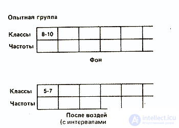
Data divided into classes on a continuous scale cannot be represented graphically as it is done above. Therefore, they prefer to use the so-called histograms, the method of graphical representation in the form of adjacent rectangles:
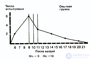
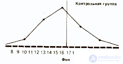
Finally, for an even more visual representation of the overall distribution configuration, it is possible to construct frequency distribution polygons . For this, segments of straight lines connect the centers of the upper sides of all histogram rectangles, and then “close” the area under the curve on both sides, bringing the ends of the polygons to the horizontal axis (frequency = 0) at points corresponding to the most extreme values of the distribution. At the same time receive the following picture:
If we compare polygons, for example, for the background (source) values of the control group and the values after exposure for the experimental group, we can see that in the first case the polygon is almost symmetrical (i.e., if you fold the polygon in half along the vertical line passing through its middle , then both halves lie on each other), whereas for the experimental group it is asymmetrical and shifted to the left (so that on its right there is a kind of elongated plume).
The polygon for the background data of the control group is relatively close to the ideal curve that could be obtained for an infinitely large population. Such a curve — the normal distribution curve — is bell-shaped and strictly symmetrical. If the amount of data is limited (as in the samples used for scientific research), then at best only a certain approximation (approximation) to the normal distribution curve is obtained.
If you build a polygon for the background values of the experimental group and the values after exposure for the control group, then you will certainly notice that this will also be the case.
If the distributions for the control group and for the background values in the experimental group are more or less symmetrical, then the values obtained in the experimental group after exposure are grouped, as already mentioned, more on the left side of the curve. This suggests that after the use of marijuana, a tendency to deterioration in a large number of subjects is revealed.
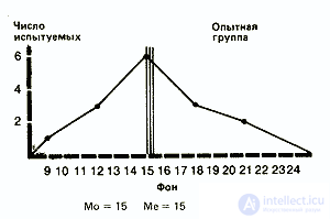
In order to express these trends quantitatively, three types of indicators are used: mode , median and average .
1. Fashion (Mo) is the easiest of all three indicators. It corresponds to either the most frequent value or the average value of the class with the highest frequency. So, in our example for the experimental group, the mode for the background will be 15 (this result occurs four times and is in the middle of the class 14-15-16), and after exposure - 9 (the middle of the class 8-9-10).
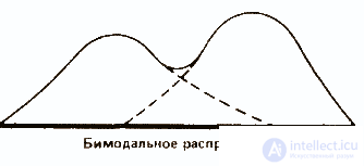
Fashion is used rarely and mainly to give a general idea of distribution. In some cases, the distribution may have two modes; then they talk about bimodal distribution. This picture indicates that in this population there are two relatively independent groups.
2. The median (Me) corresponds to the central value in the sequential series of all values obtained. So, for the background in the experimental group, where we have a number
10 11 12 13 14 14 15 15 15 15 17 17 19 20 21,
the median corresponds to the 8th value, i.e. 15. For the effects in the experimental group, it is equal to 10.
If the number of data n is even, the median is equal to the arithmetic average between the values in the row at the n / 2 and n / 2 + 1 places. Thus, for the effects for the eight young men of the experimental group, the median is between the values located at the 4th (8/2 = 4) and 5th places in the row. If you write out the entire series for this data, namely
7 8 9 11 12 13 14 16,
then it turns out that the median corresponds to (11 + 12) / 2 = 11.5 (it can be seen that the median does not correspond to any of the values obtained here).
3. Средняя арифметическая (М) (далее просто «средняя») — это наиболее часто используемый показатель центральной тенденции. Ее применяют, в частности, в расчетах, необходимых для описания распределения и для его дальнейшего анализа. Ее вычисляют, разделив сумму всех значений данных на число этих данных. Так, для нашей опытной группы она составит 15,2(228/15) для фона и 11,3(169/15) для результатов воздействия.
Если теперь отметить все эти три параметра на каждой из кривых экспериментальной группы, то будет видно, что при нормальном распределении они более или менее совпадают, а при асимметричном распределении — нет.
Прежде чем идти дальше, полезно будет вычислить все эти показатели для обеих распределений контрольной группы — они пригодятся нам в дальнейшем:
Оценка разброса
Как мы уже отмечали, характер распределения результатов после воздействия изучаемого фактора в опытной группе дает существенную информацию о том, как испытуемые выполняли задание. Сказанное относится и к обоим распределениям в контрольной группе:

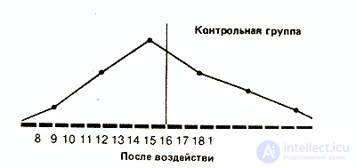
Сразу бросается в глаза, что если средняя в обоих случаях почти одинакова, то во втором распределении результаты больше разбросаны, чем в первом. В таких случаях говорят, что у второго распределения больше диапазон, или размах вариаций, т. е. разница между максимальным и минимальным значениями.
Так, если взять контрольную группу, то диапазон распределения для фона составит 22-10=12, а после воздействия 25-8=17. Это позволяет предположить, что повторное выполнение задачи на глазодвигательную координацию оказало на испытуемых из контрольной группы определенное влияние: у одних показатели улучшились, у других ухудшились. Здесь мог проявиться эффект плацебо, связанный с тем, что запах дыма травы вызвал у испытуемых уверенность в том. что они находятся под воздействием наркотика. Для проверки этого предположения следовало бы повторить эксперимент со второй контрольной группой, в которой испытуемым будут давать только обычную сигарету.
Однако для количественной оценки разброса результатов относительно средней в том или ином распределении существуют более точные методы, чем измерение диапазона.
Чаще всего для оценки разброса определяют отклонение каждого из полученных значений от средней (М-М), обозначаемое буквой d, а затем вычисляют среднюю арифметическую всех этих отклонений. Чем она больше, тем больше разброс данных и тем более разнородна выборка. Напротив, если эта средняя невелика» то данные больше сконцентрированы относительно их среднего значения и выборка более однородна.
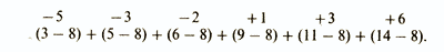
Итак, первый показатель, используемый для оценки разброса, — это среднее отклонение. Его вычисляют следующим образом (пример, который мы здесь приведем, не имеет ничего общего с нашим гипотетическим экспериментом). Собрав все данные и расположив их в ряд
3 5 6 9 11 14 ,
находят среднюю арифметическую для выборки:
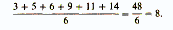
Затем вычисляют отклонения каждого значения от средней и суммируют их:
Однако при таком сложении отрицательные и положительные отклонения будут уничтожать друг друга, иногда даже полностью, так что результат (как в данном примере) может оказаться равным нулю. Из этого ясно, что нужно находить сумму абсолютных значений индивидуальных отклонений и уже эту сумму делить на их общее число. При этом получится следующий результат:
среднее отклонение равно
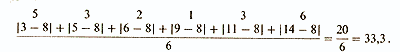
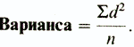
Общая формула:
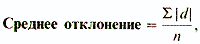
где S(сигма) означает сумму; |d| — абсолютное значение каждого индивидуального отклонения от средней; n — число данных.
Однако абсолютными значениями довольно трудно оперировать в алгебраических формулах, используемых в более сложном статистическом анализе. Поэтому статистики решили пойти по «обходному пути», позволяющему отказаться от значений с отрицательным знаком, а именно возводить все значения в квадрат, а затем делить сумму квадратов на число данных. В нашем примере это выглядит следующим образом:
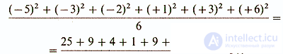
В результате такого расчета получают так называемую вариансу . (Варианса представляет собой один из показателей разброса, используемых в некоторых статистических методиках (например, при вычислении критерия F; см. следующий раздел). Следует отметить, что в отечественной литературе вариансу часто называют дисперсией. — Прим. перев.) Формула для вычисления вариансы, таким образом, следующая:
Наконец, чтобы получить показатель, сопоставимый по величине со средним отклонением, статистики решили извлекать из вариансы квадратный корень. При этом получается так называемое стандартное отклонение:
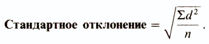
В нашем примере стандартное отклонение равно √14 = 3,74.
Следует еще добавить, что для того, чтобы более точно оценить стандартное отклонение для малых выборок (с числом элементов менее 30), в знаменателе выражения под корнем надо использовать не n , а n- 1:
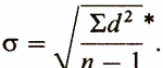
(*Стандартное отклонение для популяции обозначается маленькой греческой буквой сигма (σ), а для выборки — буквой s. Это касается и вариансы, т.е. квадрата стандартного отклонения: для популяции она обозначается σ2, а для выборки — s2.)
Вернемся теперь к нашему эксперименту и посмотрим, насколько полезен оказывается этот показатель для описания выборок.
На первом этапе, разумеется, необходимо вычислить стандартное отклонение для всех четырех распределений. Сделаем это сначала для фона опытной группы:
Расчет стандартного отклонения для фона контрольной группы
| Испытуемые | Число пораженных мишеней в серии | Average | Отклонение от средней (d) | Квадрат отклонения от средней (d2) |
| one 2 3 . . . 15 | nineteen ten 12 . . . 22 | 15.8 15.8 15.8 . . . 15.8 | -3,2 +5,8 +3,8 . . . -6,2 | 10,24 33,64 14,44 . . . 38,44 |
| Сумма (S)d2 = | 131,94 | |||

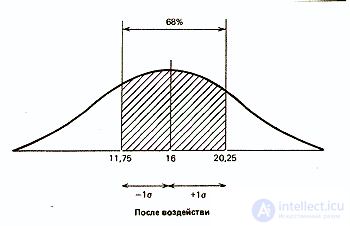
О чем же свидетельствует стандартное отклонение, равное 3,07? Оказывается, оно позволяет сказать, что большая часть результатов (выраженных здесь числом пораженных мишеней) располагается в пределах 3,07 от средней, т.е. между 12,73 (15,8-3,07) и 18,87 (15,8+3,07).
Для того чтобы лучше понять, что подразумевается под «большей частью результатов», нужно сначала рассмотреть те свойства стандартного отклонения, которые проявляются при изучении популяции с нормальным распределением.
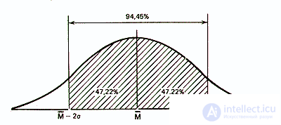
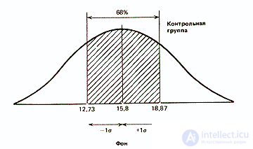
Статистики показали, что при нормальном распределении «большая часть» результатов, располагающаяся в пределах одного стандартного отклонения по обе стороны от средней, в процентном отношении всегда одна и та же и не зависит от величины стандартного отклонения: она соответствует 68% популяции (т.е. 34% ее элементов располагается слева и 34% — справа от средней):
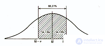
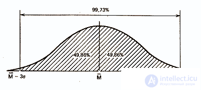
Similarly, it was calculated that 94.45% of the population elements in a normal distribution does not go beyond two standard deviations from the mean:
and that within the three standard deviations almost the entire population fits - 99.73%.
Considering that the frequency distribution of the background of the control group is fairly close to normal, it can be assumed that 68% of the members of the entire population from which the sample was taken will also receive similar results, i.e. hit approximately 13-19 targets out of 25. The distribution of the results of the other members of the population should be as follows:
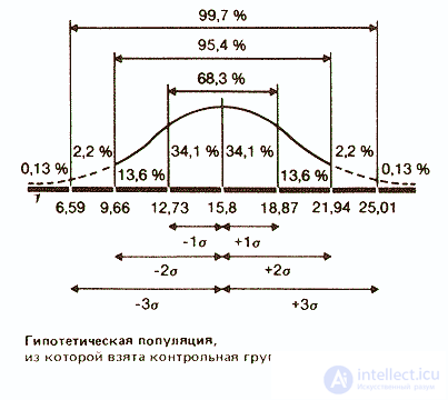
As for the results of the same group after exposure to the studied factor, the standard deviation for them was equal to 4.25 (affected targets). Therefore, it can be assumed that 68% of the results will be located in this range of deviations from the average, which is 16 targets, i.e. ranging from 11.75 (16-4.25) to 20.25 (16 + 4.25), or, rounding off, 12 to 20 targets out of 25. It can be seen that here the scatter of results is greater than in the background. This difference in the spread between the two samples for the control group can be represented graphically as follows:
Since the standard deviation always corresponds to the same percentage of results that fit within its limits around the average, it can be argued that for any form of the normal distribution curve, that fraction of its area that is limited (on both sides) by the standard deviation is always the same and corresponds to one and the same proportion of the entire population. This can be checked on those samples for which the distribution is close to normal, on the background data for the control and experimental groups.
So, having familiarized ourselves with descriptive statistics, we learned how it is possible to graphically represent and quantify the degree of data spread in a given distribution. Thus, we were able to understand the differences in our distribution experience for the control group before and after exposure. However, is it possible to judge something by this difference - does it reflect reality or is it just an artifact associated with too small a sample size? The same question (only more acutely) arises in relation to the experimental group subjected to the influence of an independent variable. In this group, the standard deviation for the background and after exposure also differs by about 1 (3.14 and 4.04, respectively). However, there is a particularly large difference between the average - 15.2 and 11.3. On the basis of what it could be argued that this difference in averages is really reliable, i.e. is large enough to be explained with confidence by its influence of an independent variable, and not by mere chance? To what extent can we rely on these results and distribute them to the entire population from which the sample was taken, that is, to say that the consumption of marijuana actually leads to a violation of eye movement coordination?
All these questions and tries to answer inductive statistics.
The tasks of inductive statistics are to determine how likely it is that two samples belong to the same population.
Let's overlap, on the one hand, two curves - before and after exposure - for the control group and, on the other hand, two similar curves for the experimental group. The scale of the curves should be the same.
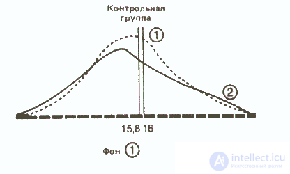
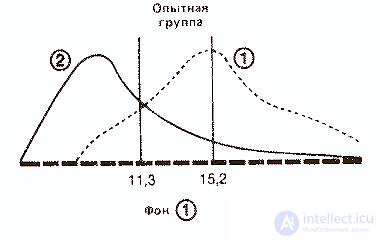
It can be seen that in the control group the difference between the averages of both distributions is small, and therefore it can be assumed that both samples belong to the same population. On the contrary, in the experimental group, the large difference between the means suggests that the distributions for the background and the impact belong to two different populations, the difference between which is due to the fact that one of them was influenced by an independent variable.
As already mentioned, the problem of inductive statistics is to determine whether the difference between the means of the two distributions is large enough so that it can be explained by the action of an independent variable, rather than an accident, associated with a small sample size (as it seems to be the case with the experimental group of our experiment).
There are two possible hypotheses:
1) the null hypothesis (H0) , according to which the difference between the distributions is unreliable; it is assumed that the difference is not significant enough, and therefore the distributions belong to the same population, and the independent variable has no effect;
2) alternative hypothesis (Hx) , which is the working hypothesis of our study. In accordance with this hypothesis, the differences between the two distributions are quite significant and are due to the influence of an independent variable.
The basic principle of the hypothesis testing method is that the null hypothesis H0 is put forward in order to try to disprove it and thereby confirm the alternative hypothesis H1. Indeed, if the results of the statistical test used to analyze the difference between the averages are such that they allow H0 to be discarded, this will mean that H1 is true, that is, The proposed working hypothesis is confirmed.
In the humanities, it is generally accepted that the null hypothesis can be rejected in favor of an alternative hypothesis if, according to the results of a statistical test, the probability of an accidental occurrence of the found difference does not exceed 5 out of 100. You can not discard the null hypothesis.
In order to judge what the probability of a mistake is by accepting or rejecting the null hypothesis, statistical methods are applied that correspond to the characteristics of the sample.
Thus, for quantitative data with distributions close to normal, parametric methods are used, based on such indicators as mean and standard deviation. In particular, the Student method is used to determine the accuracy of the difference between the averages for two samples, and to judge the differences between three or more samples, test F, or analysis of variance.
If we are dealing with non-quantitative data or the samples are too small to be sure that the populations from which they are taken are subject to a normal distribution, then non - parametric methods are used — the χ 2 (chi-square) criterion for qualitative data and the criteria for marks, ranks , Mann-Whitney, Wilcoxon and others for ordinal data.
In addition, the choice of a statistical method depends on whether the samples that are compared are independent (that is, for
продолжение следует...
Часть 1 Statistics and data processing in psychology
Часть 2 Levels of confidence (significance) - Statistics and data processing in
Часть 3 - Statistics and data processing in psychology

Comments
To leave a comment
Mathematical Methods in Psychology
Terms: Mathematical Methods in Psychology