Lecture
Introduction
Multidimensional scaling began its intensive development in the 60s in the works of American scientists Thorgerson (Torgerson) [9], Shepard (Shepard) [8], and Kruskal [6]. The circle of Soviet specialists dealing with this problem is rather narrow, and their main efforts are aimed at developing formalized methods and computational procedures that implement known models on a computer. To date, the methods of multidimensional scaling, unfortunately, are not widely used in psychometric studies in our country. Apparently, the reasons for this are the small number of specialists and the lack of good software packages.
The development of multidimensional scaling goes in the direction of its increasingly formalization. At the same time, some substantive issues remain in the shadow, the discussion of which could attract the attention of a large number of users and would contribute to the expansion of the field of application of these methods. Not enough attention is paid to studying the properties of multidimensional scaling models. There are no publications (including available American sources) in which the scaling mechanism itself would be analyzed and how the methods of multidimensional scaling allow to single out the factors taken into account by a person when comparing stimuli. These questions are directly related to the problem of a meaningful interpretation of a formally constructed solution.
This paper attempts to explain the geometric properties of multidimensional scaling models and demonstrates the possibilities of using them for the analysis of subjective perception.
The task of multidimensional scaling in the most general form is to identify the structure of the studied set of stimuli. Identifying a structure is understood as highlighting a set of main factors by which incentives differ, and describing each of the incentives in terms of these factors. The procedure of building a structure is based on the analysis of objective or subjective information about the proximity between stimuli or information about preferences on a variety of stimuli. In the case of analysis of subjective data, two problems are solved simultaneously. On the one hand, an objective structure of subjective data is revealed, on the other hand, factors influencing the decision-making process are determined.
Multidimensional scaling methods can use different types of data: data on the preferences of the subject on a set of stimuli, data on dominance, on proximity between stimuli, data on profiles, etc. As a rule, it is customary to correlate a certain group of processing methods with each data type. However, this correlation should not be too hard, since it is often not difficult to move from one type of data to another. For example, profile data can be easily converted to proximity data, for this it is only necessary to use a suitable metric. Preference data contains information about dominance. On the other hand, by calculating the correlations between the columns of the matrix of preferences, we obtain a matrix of intimacy between stimuli, and correlations between the rows of the same matrix will give us a matrix of intimacy between subjects. In this paper, only the proximity analysis will be discussed.
The basis of multidimensional scaling is the idea of the geometric representation of the stimulus set. Suppose we are given a coordinate space, each axis of which corresponds to one of the required factors. Each stimulus is represented by a point in this space, the magnitudes of the projections of these points on the axis correspond to the values or powers of the factors characterizing the given stimulus. The greater the magnitude of the projections, the greater the value of the factor the stimulus has. The measure of similarity between two stimuli is inverse to the distance between the points corresponding to them. The closer the stimuli are to each other, the higher the measure of similarity between them (and the lower the measure of difference), the farthest points correspond to the low measure of similarity. In order to accurately measure proximity, you must enter the metric in the desired coordinate space; The choice of this metric has a great influence on the result of the decision.
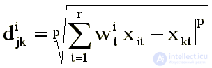
Commonly used Minkowski metric:
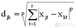
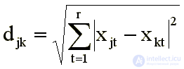
where r is the dimension of space, djk is the distance between points corresponding to the jth and kth stimuli, Xjt , Xkt are the values of the projections of the jth and kth points to the tth axis. Its most common cases are: Euclidean metric (p = 2):
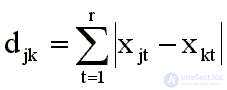
and metric "city-block" (p = 1)
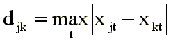
In some cases, use the dominance metric (p tends to infinity):
The use of uniform metrics implies that when assessing the similarities (differences) the subject equally takes into account all factors. When there is reason to assert that factors are unequal for an individual and he takes them into account in varying degrees, they resort to a weighted metric, where a certain weight is attributed to each factor. Different individuals may take different factors into account. Then each individual is characterized by its own set of weights Wti . The weighted Minkowski metric is:
Such a model is called “individual scaling” or “model of weighted factors” [2, 12, 13]. Geometrically, it is interpreted as follows. Let in the coordinate space there is a configuration of points reflecting the perception of some “average individual” in the group. In order to obtain the perceptual space of the i-th subject, it is necessary to stretch the “average configuration” in the direction of those axes for which Wti> Wtcp , and compress in the direction of the axes for which Wti <Wtср . For example, if in the space of two factors for an “average individual” all incentives lie on a circle, then for an individual characterized by weights W1i = 2, W2i = 1, these incentives will be located on an ellipse stretched along the horizontal axis, and for an individual characterized by weights W2i = 2, W1i = 1, on an ellipse stretched along the vertical axis.
The multidimensional scaling scheme includes a series of successive stages. At the first stage, it is necessary to obtain in an experimental way subjective assessments of the differences. The survey procedure and the type of assessment should be chosen by the researcher depending on the specific situation. As a result of this survey, a subjective matrix of pairwise differences between stimuli should be constructed, which will serve as input for the next stage.
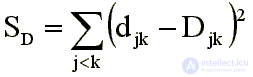
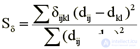
At the second stage, the problem of constructing the coordinate space and placing stimulus points in it is solved in such a way that the distances between them, determined by the entered metric, best fit the original differences between the stimuli. To solve this formal problem, no information is needed about the stimuli themselves; it is enough to have only a matrix of pairwise differences between them. To construct the desired coordinate space, a sufficiently developed apparatus of linear or nonlinear optimization is used. A mapping quality criterion, called “stress,” is introduced that measures the degree of discrepancy between the initial differences Djk and the resulting distances djk . Looking for a configuration of points that would give the minimum value of this "stress." The coordinates of these points are the solution to the problem.
Using these coordinates, we construct a geometric representation of the stimuli in a space of a low number of dimensions. It must be sufficiently adequate to the source data. The incentives to which large measures of difference correspond in the initial matrix should be far from each other, and the incentives to which small measures of difference correspond should be close. The formal criterion of adequacy can serve as a correlation coefficient, it should be quite high. The means of increasing the accuracy of a formal solution is to increase the number of dimensions, that is, the dimension of the space r . The higher the dimension of space, the more opportunities to get a more accurate solution.
The geometric representation of stimuli in a space of a small number of dimensions is the result of independent significance. It will provide an opportunity for visual presentation of data convenient for visual analysis, and the directions for its use go far beyond psychometric research.
At the third stage, the substantive task of interpreting the formal result obtained at the previous stage is solved. The coordinate axes of the constructed stimulus space should receive a semantic content, they should be interpreted as factors determining the differences between the stimuli. This work is quite complex and can only be performed by a specialist familiar with the material under study. If at the previous stage there was only enough information on pairwise differences between stimuli, then a thorough study of their characteristics is necessary for meaningful interpretation.
The multidimensional scaling offers a geometric representation of the stimuli in the form of points of the coordinate space of the smallest possible dimension.
There are two types of models: distance and vector. In remote models, the original differences should be approximated by distances, in most cases using the usual Euclidean distance:
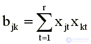
In vector models, measures of proximity or connections are the inverse of the difference, approximated by scalar products of vectors connecting the points corresponding to the stimuli with the origin:
When building a configuration of incentives, a linear or non-linear optimization apparatus is used. Why does such a simple model and formal methods for finding extremums allow us to get a meaningfully interpreted solution? Why do axes constructed in a formal way acquire the meaning of well-interpreted factors?
Vector model. Let's discuss the geometric properties of the vector model. Let's start with the scaling of binary data, i.e. statements like "similar - unlike". Assume that we have a matrix containing information that all incentives are not similar to each other. How can one imagine such a structure geometrically? Incentives should be located either on orthogonal straight lines, or at the origin. In this case, all scalar products will be zeros.
Let us turn to the situation of the presence of several groups of similar incentives. Incentives from one group should be represented by one point; points corresponding to different groups must belong to orthogonal straight lines. Isolated stimuli can be placed at the origin. Then the scalar products between similar stimuli will be large, and the scalar products between dissimilar stimuli will be zeros.
Orient the axes of the coordinate space along orthogonal directions. Then each axis will be associated with a group of similar incentives, and the corresponding factor will underlie the similarity of these incentives. Different groups will correspond to orthogonal pox and, therefore, independent factors. The exceptions are isolated stimuli that can get to the origin. The more incentives are grouped, the less measurements are needed.
Let now we have discrete or continuous data, t. we obtain estimates of similarities or connections, either in the form of points or in the form of numbers. Suppose that in this case the matrix has a quasi-block structure. Then, according to it, the whole set can be divided into several groups so that the incentives within each group will be strongly connected, and the incentives from different groups are weakly connected with each other. The character of the mapping will be about the same as in the case of disjoint binary data. However, incentives from one group will not be represented by one point, but will be concentrated in some of its surroundings. Such a structure, generally speaking, will not coincide with an orthogonal coordinate system, since points may lie somewhat away from the axes. However, if the links in the groups are strong enough, and the links between the groups are weak enough, then in this case each measurement will be associated with one group and the corresponding factor will underlie the similarity of incentives from this group.
In practice, highly structured data characterizing non-overlapping groups of stimuli are rare, usually the groups have intersections. There are incentives that are simultaneously similar to incentives from two or more groups. Naturally, they will not fall on the axis, but will be located in the space between them. The nature of the distribution will depend on the matrix of source data. The picture will be all the more contrasted, the more structured the data is, i.e., the intra-group ties are stronger and the inter-group links are weaker. Axes will be determined by groups of incentives that are very similar to each other and minimally similar to incentives from other groups. Such incentives are characterized by large values of coordinates along the corresponding axes. These groups of incentives underlie the whole structure. The rest of the incentives, similar to the incentives from several groups at the same time, should occupy intermediate positions between these groups.
Since the original matrix is not a matrix of exact distances or scalar products, all stimuli cannot be displayed in the space defined by the orthogonal axes corresponding to isolated groups. For their placement will require additional dimensions. If the first type of dimensions is determined by large intergroup differences and each dimension is characterized by a significant range of stimuli, the second type of dimensions arises due to the fact that the subjective differences between the stimuli cannot be displayed accurately in the space of a small number of dimensions. The spread of stimuli along the dimensions of the second type is small and in many cases it can be neglected.
Centered vector model. Another variant of the vector model is the model of centered scalar products. It is based on the widely used Thorgerson method, which initiated the theory of multidimensional scaling. In this model it is assumed that the origin of the coordinates is placed in the center of gravity of the structure. The initial proximity or connections should be approximated by scalar products of vectors connecting the points corresponding to the stimuli with the center of gravity of the configuration. The matrix of initial proximity is pre-centered, so that along with positive numbers, negative ones also appear in it. If we normalize the given data: | ajk | Ј1, then they can be considered as correlation coefficients.
The solution generated by the model of centered scalar products differs from the solution obtained by the usual vector model. In the original matrix of proximity (communication) between stimuli can take positive, zero and negative values; we will approximate them with scalar products. Naturally, incentives characterized by strong positive connections (large measures of proximity) should be concentrated in the vicinity of one point, located at a considerable distance from the origin. Then the scalar products between the corresponding vectors will be large. Incentives characterized by negative connections should be located on opposite sides of the origin. Scalar products between them will take the maximum negative values if they belong to different ends of one straight line passing through the origin. Pairs of stimuli with zero coupling must belong to orthogonal straight lines; in this case, the scalar products between them will be zeros. Isolated stimuli that have zero links with everyone else can fall at the origin.
Large positive, negative, and zero connections will determine the basic structure of the entire system. Incentives characterized by moderate connections will be located between these main groups of incentives. The weaker the connections, the closer the incentives to the top coordinates. Since the initial matrix of proximity or connections is not an exact matrix of scalar products, all stimuli cannot be displayed in a space of small dimension. As in the case of the previous model, to compensate for the noise in the data, additional dimensions will be required, the spread in the direction of which is insignificant compared to the main dimensions and can be neglected. Thus, the model of centered scalar products allows to display the structure of the system in the coordinate space spanned by a small set of orthogonal lines. Rotate the original axes of space and combine them with these straight lines. Then each axis can be interpreted as a bipolar factor: there will be stimuli on the right, characterized by positive values of this factor, on the left - negative, and in the center - zero.Orthogonal axes will correspond to stimuli or groups of stimuli that are not related to each other, so they can be interpreted as independent factors. The solution generated by the model will have a semantic content.
Remote model Let us now see what properties the remote model has; we restrict ourselves to the Euclidean metric. Let's start again with a system in which all incentives are not similar to each other. To accurately transfer the structure of this system, each stimulus should be placed in one of the N vertices of the polyhedron with the same edges (simplex). Then the stimuli will be equally spaced apart.
Пусть имеется несколько изолированных групп- стимулов. Тогда стимулы из одной группы должны быть помещены в одну вершину, и многогранник будет иметь размерность, равную количеству групп. В отличие от векторной модели изолированные стимулы не могут быть все помещены в одну точку — начало координат, каждый из них должен занимать отдельную вершину.
В общем случае произвольной матрицы различий группы похожих между собой стимулов будут сконцентрированы вблизи одной вершины, а стимулы, похожие одновременно на стимулы из двух или нескольких групп, будут располагаться между этими вершинами.
Характер конструкции будет определяться в основном большими различиями между стимулами или группами стимулов. Однако, как и в случае векторной модели, ввиду того, что матрица различий не является точной матрицей расстояний, для передачи структуры потребуются дополнительные размерности. Но разброс стимулов в этих направлениях будет сравнительно мал.
В результате шкалирования необходимо выявить существенные оси, разброс в направлении которых велик, и отбросить несущественные оси, разброс в направлении которых мал. Итак, следуя модели многомерного шкалирования, можно разместить все стимулы в пространстве таким образом, чтобы оси несли смысловую нагрузку и факторы, им соответствующие, лежали в основе сходств или различий между стимулами.
Построенная результирующая конфигурация и полученные размерности отражают данные, занесенные в матрицу близостей или различий. И хотя многомерное шкалирование при своем зарождении было предназначено для анализа высказываний человека, никакой специфики обработки субъективных данных в нем не содержится. Оно в равной мере может использоваться и для анализа объективных данных о близостях или связях. Более того, иногда легче поддаются интерпретации объективные данные, потому что они характеризуют некие объективные связи между объектами. Интерпретация субъективных данных, построенных на основе высказываний одного человека (эксперта, испытуемого), может вызвать значительные затруднения у другого человека (исследователя, экспериментатора).
После анализа механизма шкалирования легко понять, какие же данные следует считать хорошими или, как принято говорить, хорошо структуризованными. Для кластерного анализа хорошо структуризованной является матрица, которая может быть приведена к блочно-диагональному виду. Иными словами, если имеется группа похожих (или сильно связанных) между собой стимулов, то все стимулы этой группы должны быть непохожими на остальные (или слабо связаны). Тогда структура может быть представлена изолированными группами сходных между собой стимулов. В многомерном шкалировании ввиду непрерывности измерений требования на входную информацию более слабые. Если два стимула сходны между собой, то они должны иметь близкие профили сходств со всеми другими стимулами. Это является необходимым условием для их адекватного представления в пространстве небольшого числа измерений.
Хотя модель многомерного шкалирования достаточно проста и интуитивно понятно, какого характера решение следует ожидать, попытки построить конфигурацию точек вручную могут привести к успеху лишь при очень небольшом количестве стимулов и хорошо структуризованной матрице близостей. В общем случае исследователь вынужден прибегнуть к помощи вычислительной машины, а для работы на ней необходимо алгоритмизировать процесс решения задачи. Иногда трудно вручную построить конфигурацию даже для небольшого набора стимулов. Примером такого множества могут служить равнояркие цветовые стимулы, равномерно распределенные по длине волны. Анализ матрицы субъективных различий не позволяет выделить ключевые стимулы, различия между которыми могли бы быть положены в основу всей структуры. Обработка этих данных на ЭВМ приводит к представлению стимулов на окружности — «цветовом круге»; действительно, с точки зрения такой структуры все стимулы равноценны.
Известны три подхода к шкалированию: линейный, нелинейный и неметрический. Линейный подход, предложенный Торгерсоном [9], основан на ортогональном проектировании в подпространство, образованное направлениями, характеризующимися значительным разбросом точек. Такое решение дает maxеd2jk при ортогональном проектировании.
В нелинейном случае [1, 7, 11] пытаются найти отображение D ® d, которое бы минимально искажало исходные различия Djk. Вводится критерий качества отображения, называемый «стрессом» и измеряющий степень расхождения между исходными различиями Djk и результирующими расстояниями djk. С помощью аппарата нелинейной оптимизации ищется конфигурация точек, которая давала бы минимальное значение «стрессу». Значения координат этих точек и являются решением задачи. В качестве «стресса» используются разные виды функционалов, в простейшем случае
The nonlinear approach, as a rule, leads to a space of a smaller dimension than the linear one. In the linear case, the distortion is allowed only in the direction of reducing the differences. In non-linear - distortion is possible both in that and in the other direction. The prerequisites for obtaining a low-dimensional mapping in space can be created by assuming the possibility of some increase in large distances and a decrease in small ones.
Неметрический (или монотонный) подход в своей последней модификации [4, 6] основан на следующем соображении. Поскольку исходная матрица различий не является точной матрицей расстояний в каком-либо метрическом пространстве, то не следует стремиться аппроксимировать непосредственно эти различия. Нужно подобрать такую последовательность чисел, которая была бы монотонна с исходными различиями, но была бы более близка к точным расстояниям. Эту последовательность чисел уже можно использовать в качестве эталонной. Однако не известен способ построения такой последовательности с учетом лишь первоначальных различий. Предлагается многоэтапная процедура, использующая начальную конфигурацию точек. На первом этапе подбирается числовая последовательность {  }, монотонная с исходными различиями и минимально отклоняющаяся от расстояний начальной конфигурации. Затем ищется новая конфигурация, расстояния которой в наилучшей мере аппроксимируют числовую последовательность { }. На втором этапе опять подбирают новую последовательность { } и конфигурацию изменяют так, чтобы ее расстояния приближали эту последовательность, и т. д. Таким образом, в качестве критерия, измеряющего качество отображения, используется функционал вида
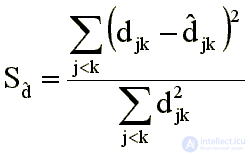
Нормирующий множитель 1/еd2jk вводится для того, чтобы на качество решения не влиял масштаб конфигурации.
Известен еще один подход к шкалированию [5], сохраняющий монотонность отображения и не опирающийся на какую-либо числовую последовательность. Он основан на минимизации критерия
Где
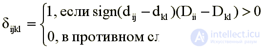
Передвижение точек конфигурации направлено на усиление монотонности отображения, т. е. удовлетворение требования dij Ј dkl, если Dij Ј Dkl.
Нелинейный и неметрический подходы имеют преимущество перед линейным. Не ограничиваясь ортогональным проектированием, они позволяют получить хорошее отображение в пространстве меньшего числа измерений. Если размерность пространства оценена правильно, то после вращения координатные оси могут быть интерпретированы как факторы, лежащие в основе субъективных различий между стимулами. Если же размерность недооценена, то решение допускает интерпретацию только в терминах кластеров.
Нелинейные и неметрические методы опираются, как правило, на дистанционную модель: различия между стимулами приближаются расстояниями между соответствующими им точками. Для поиска решения они используют градиентные процедуры минимизации функционала. В большинстве случаев расстояния между точками вычисляются по евклидовой метрике, которая не чувствительна к вращению осей и переносу начала координат. Качество решения не зависит от направления системы координат, по этой причине формально полученные оси не могут нести смысловую нагрузку — для содержательной интерпретации они должны быть ориентированы соответствующим образом.
В основу линейного метода Торгерсона положена центрированная векторная модель: близости между стимулами должны быть аппроксимированы скалярными произведениями векторов, соединяющих точки-стимулы с центром тяжести структуры. Решение ищется путем факторизации матрицы исходных близостей (или связей); вычисляются ее собственные значения и собственные векторы. Такая процедура обусловливает жесткую ориентацию осей: первая ось характеризуется максимальным разбросом точек вдоль нее, вторая — ортогональна первой и определяется следующим по величине разбросом, третья — ортогональна плоскости первых двух и т. д. В тех практических ситуациях, когда существует фактор, по которому стимулы различаются больше, чем по всем остальным, первая ось будет соответствовать этому фактору. В таком случае формально полученные оси будут иметь смысловое содержание. Если же с точки зрения вклада в различия между стимулами все факторы или несколько из них равноценны, то для интерпретируемости осей необходимо произвести их поворот.
Многомерное шкалирование по своему происхождению является областью математической психологии и первая его задача — это анализ субъективного восприятия. Методы многомерного шкалирования можно использовать для построения модели поведения человека при вынесении суждений о сходстве между различными стимулами. Процесс оценки субъектом сходств между стимулами может быть представлен в виде традиционного «черного ящика», на вход которого подается информация о стимулах, а на выходе получают субъективные высказывания о сходствах. Задача состоит в том, чтобы описать этот «черный ящик». Под моделью понимается система правил, руководствуясь которой, можно генерировать те же результаты о сходствах, какие были высказаны субъектом для анализируемого набора стимулов.
В основе модели лежит предположение о том, что при сравнении стимулов человек (явным или неявным образом) сопоставляет их характеристики. Чем сильнее расхождение стимулов по этим характеристикам, тем выше субъективная мера различия между ними. Следовательно, задача сводится к тому, чтобы для исследуемого множества стимулов 1) выявить набор основных факторов, их характеризующих, 2) описать каждый стимул с помощью этих факторов и 3) сконструировать функцию, позволяющую определить меру различия между стимулами на основе известных значений по факторам.
Четвертый заключительный этап включает процедуру построения модели принятия решений о сходствах, использующую параметризацию стимулов с помощью выделенных факторов и их геометрическое представление в пространстве этих факторов. Нужно описать «черный ящик», т. е. в терминах расстояний между стимулами сформулировать правило, следуя которому можно получить те же меры сходств, которые получены от субъекта в ходе эксперимента. Необходимо также оценить степень адекватности модели субъективным данным. Для большей наглядности результата кроме коэффициента корреляции можно использовать также корреляционное поле. Чем большее количество факторов принимается во внимание при построении модели, тем, конечно, она лучше приближает исходные данные. Наша цель, однако, ограничиться минимальным набором факторов, достаточным для построения модели, адекватной анализируемым субъективным сходствам (различиям).
Многомерное шкалирование предоставляет формальный способ построения модели, основывающийся только на результирующих высказываниях субъекта. Такой способ может использоваться, когда человек опирается на свою интуицию и не может описать процесс принятия решения. Заметим, что мы будем строить «апостериорную» модель. Это означает, что мы можем начать работу только после того, как получим от субъекта информацию о сходствах, и попытаемся объяснить, какими мотивами он руководствовался при вынесении своих суждений. Поэтому, строго говоря, наша модель будет верна только для набора стимулов, участвующих в эксперименте. Но если предъявляемая выборка окажется достаточно представительной, то построенная модель будет обладать прогностической силой и по ней можно будет предсказывать, какие решения будет принимать субъект, если в эксперимент будут включены другие стимулы, подобные анализируемым.
Пятидесяти субъектам предъявлялись попарно восемнадцать букв русского алфавита, и они оценивали близость в каждой паре в терминах «похожи—непохожи». В результате [3] были получены пятьдесят матриц сходств, которые затем были обработаны методом многомерного шкалирования. Анализ конфигурации, приведенной на рис. 1, позволяет, во-первых, выделить группы букв, сходных с точки зрения субъектов, и, во-вторых, выявить два фактора, которыми руководствовались субъекты при вынесении суждений о сходствах. Легко различить три «чистых» группы букв, состоящих из остроугольных элементов (К, У, М. Л, А, И), из прямоугольных элементов (И, П, Д, Т, Г, Е), из круглых элементов (О, С), и одну «смешанную», состоящую из букв, включающих элементы двух типов—прямые и круглые (Б, В, Р), и расположенную между группой букв из круглых элементов и группой букв из прямоугольных элементов. Промежуточное положение заняла буква 3, она расположилась между группой круглых и группой комбинированных букв, в частности из последних ближе всего к В. Буква Е заняла в группе прямых крайнюю позицию, примыкая к комбинированным Б и В.
As for the factors, one of them was possible to interpret as the presence of only direct elements — the presence of only round elements; in the middle are the letters consisting of straight and round elements at the same time. The second factor is interpreted as the presence of acute-angled elements - the presence of rectangular elements.
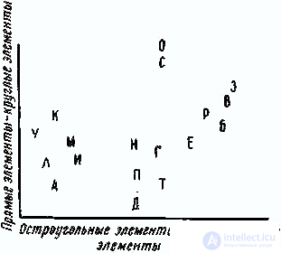
Fig. 1. Analysis of visual perception. Incentive space
The analysis of weights leads to the following conclusions. First, the subjects differ in how much weight they give to each of the factors. So, one part of the subjects gave a lot of weight to the horizontal axis, the other - to the vertical one. At the same time, for different subjects the degree of difference in weights varies. Much of them are grouped along the diagonal, for these subjects the difference between weights is insignificant. At the same time, for subject No. 47, the weights differ very much - he ascribes significantly more weight to the horizontal axis than to the vertical one. For subject 41, this difference is also very large, but for him the first weighting factor is significantly less than the second. Thus, while subject No. 47, in assessing the similarity between letters, is guided mainly by the presence or absence of acute-angle elements in them, subject No. 41 mainly takes into account only the presence or absence of round elements.
In addition to the difference in the ratio of two weights between subjects, there is a difference in their magnitude. Direct analysis of the original matrices shows that subjects who, when comparing pairs of letters gave both factors small weights, correspond to a large number of answers “similar”, and subjects who gave both factors greater weights correspond to the greatest number of answers “unlike”.
The naturalness of the constructed model is illustrated by the following example. Consider several letters that did not participate in the experiment, for example, the letters Ж, X, Ш, Я. Obviously, Ж and Х should be attributed to the class of acute-angled letters, W - to the class of letters with right angles. The letter I can not be attributed to any of the classes obtained, but its position in the space of two signs can be clearly defined. In the first factor, it takes place at the level of letters containing both straight and round elements (such as P, B), and in the second, at the level of letters with sharp corners (K, Y). Thus, the letter I can be characterized as consisting of both round and straight elements and containing acute angles. Thus, according to our model, it is possible to predict the results of future experiments without conducting them.
In Bulgaria at the Institute for Teaching Foreign Students to the Bulgarian Language, studies were conducted on the differences in the perception of Bulgarian sounds between Bulgarians and foreign students [10]. Were selected four groups of subjects for 50 people: Bulgarians, Spaniards, Vietnamese and Arabs. Pairs of 21 consonants in combination with b (Bb – Bb) were recorded on magnetic tape — a total of 210 pairs. The subjects had to listen carefully and note whether the two sounds in a pair are similar. As a result, a matrix of similarities was obtained for each subject.
A joint analysis of these data allowed us to construct a six-dimensional stimulus space. 1st axis (fig. 2) divides all consonants into sibilants
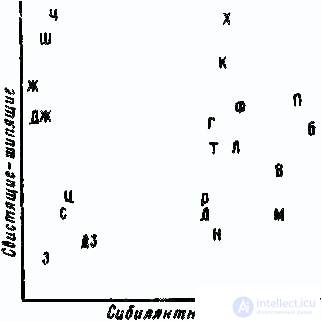
Fig. 2. Analysis of hearing. The stimulus space is the plane formed by the 1st and 2nd axes
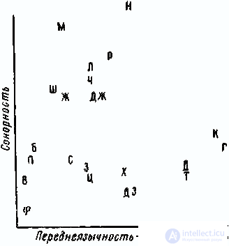
Fig. 3. Analysis of hearing. The stimulus space is the plane formed by the 3rd and 4th axes
(H, Sh, F, J, C, C, 3, DZ) and the rest. 2nd axis separates sibilants by frequency: high-frequency - whistling (3, C, C, DZ) and low-frequency - hissing (H, W, F, DJ). The 3rd axis (Fig. 3) distinguishes from all consonants the sonor group (M, H, L, P); 4th corresponds to the place of formation of sounds: from the labial to the back-lingual. The first level is composed of lip sounds (P, B, B, F, T), the second is dental (C, H, C, L, 3, F, J, N, DZ), the third is frontal (T, D) and the fourth - rear lingual (K, D). The 5th axis highlights the quivering sound of R. The 6th axis is interesting, it corresponds to the sign “deafness - voicing”, but “quantity of voicing” is defined as if in a relative degree; the opposition of “deafness to voicing” is realized on all consonants, but in pairs: C lies farther from the origin of coordinates than 3; W - further than F; H - further than JJ, etc. The same is true for the pairs T – D, P – B, K – D, F – C.
All subjects, and especially the group of Spaniards, when comparing sounds, give the greatest importance to the attribute “sibilance”. For the Spaniards are also characterized by large weights for the sign of "sonority." The Arabs have the lowest weights, they take into account the signs “whistling - hissing”, “sonorous - non-sensory”, “deaf - ringing”. The Bulgarians, to a lesser extent than all the others, take into account the sign “front-lingual — rear-lingual”, but when comparing, they mostly rely on the sign “deaf-sounded - voiced.” Apparently, the difference in the perception of sound stimuli by different groups of subjects - carriers of different languages - is explained by the difference in phonetic systems that their native languages rely on.
Conclusion
Multidimensional scaling methods are designed to analyze the structure of subjective data. They make it possible to identify the factors underlying the similarities and differences between incentives, and to construct a model for making decisions about similarities. It should be noted that the methods of multidimensional scaling work only in the case when the similarities or differences between all the stimuli of the studied set are generated by a single regularity. When comparing one pair of incentives, the subject relies on one system of factors, and when comparing the other pair on another, multidimensional scaling cannot give a satisfactory result. In addition, the decision will significantly depend on the proposed set of incentives (context). The same incentives included in different sets can be described by different factors. This circumstance is a consequence of the fact that the differences between the stimuli of one set may be characterized by differences in one factor, and the differences between the stimuli of another set - differences in other factors. So, if we show the subject stimuli of the same shape but different colors, he will only pay attention to the color when comparing. If at the same time we vary the form of stimuli, then the subject will also take into account the form. Let us once again emphasize that using the proposed multidimensional scaling procedure, we can reveal only those factors by which the stimuli of the test set differ, but it is impossible to identify the factors by which they are all similar.
Literature
Psychological Journal, Volume 4, №1. - 1983. - P.76-88

Comments
To leave a comment
Mathematical Methods in Psychology
Terms: Mathematical Methods in Psychology