Lecture
Published according to the monograph by V. A. Duke
"Computer psychodiagnostics", (S-Pb., 1994)
Introduction
Of great importance in the development of experimental psychodiagnostic methods are technical means of stimulating, recording and processing psychodiagnostic information. These technical tools have found their most complete embodiment in modern high-performance computers with their powerful operational and visual capabilities.
The use of modern computers in psychodiagnostics of possibilities for compact storage, quick retrieval, promptly and comprehensively analyze and clearly display experimental information entails effects that can be called quantitative and qualitative.
The first type of quantitative effects is mainly related to automating the routine operations of a traditional psychodiagnostic experiment, such as instructing the subject, presenting stimuli and recording the subject's answers, keeping a protocol, calculating and delivering results, etc. The level of standardization, accuracy and speed are increased by such automation. obtaining diagnostic output, which is extremely necessary in areas such as clinical examination or psychological counseling. In addition, the speed of information processing in a computer experiment allows mass psychodiagnostic examinations to be carried out in a short time, which, in particular, are used to solve problems of professional psychological selection or vocational guidance in the conditions of shortage of time and other resources.
Qualitative effects can be divided into two categories. The first category consists of the effects provided by the capabilities of modern computers to implement new types of psychodiagnostic experiments. These include the ability to generate new types of stimuli (dynamic and polymodal), reorganize the stimulus sequence (for example, the so-called adaptive testing), register previously unavailable reaction parameters of the subjects, design psychodiagnostic techniques in the form of computer games, etc. Second category qualitative effects are associated with the use in psychodiagnostics of the latest advances in information technology. These achievements concern the methods of creating and maintaining computer databases, pattern recognition algorithms in psychodiagnostics, and artificial intelligence methods based on the manipulation of knowledge in the subject domain under consideration.
Consider the external side of a typical procedure of "manual" data processing psychodiagnostic testing.
The subject returns to the psychologist a survey form on which his chosen answers to the questions (tasks) of the psychodiagnostic test are marked. The psychologist calculates the number of "hits" of the answers of the subject in accordance with the diagnostic "key". Then the psychologist using tables or nomograms translates the calculated amount into a new number - a standardized estimate. This assessment or several assessments defined in a similar way are the result of psychodiagnostic testing, which allows the psychologist to make a judgment about the characteristics of the subject, to make a certain forecast for the future and to give certain recommendations.
The described procedure for converting a test subject's answers into a diagnostic indicator underlies the majority of psychodiagnostic tests. Known more complex ways of compiling primary diagnostic information. But already behind this seemingly simple measuring procedure is the painstaking work of the creator of the psychodiagnostic test, associated with obtaining and time-consuming analysis of experimental psychological data. Some types of such analysis can be performed manually or with the help of a micro calculator. However, a truly deep empirical-statistical analysis that provides reasonable, accurate and reliable diagnostic results is inconceivable without the use of modern computer methods.
In the work of the researcher on the design of psychodiagnostic test, there are three main stages.
At the first stage, the experimenter, proceeding mainly from theoretical ideas about the construct being diagnosed, forms the “draft” version of the test. This option includes tasks, the answers to which, in the opinion of the experimenter, should reflect the individual psychological differences of the subjects on a given construct. The definition of a “draft” version of the psychodiagnostic test (the initial set of diagnostic features) is a difficult task to formalize. Therefore, in the framework of this chapter, only the most general recommendations on the formation of the initial set of diagnostic features will be given.
At the second stage, the researcher chooses a diagnostic model and determines its parameters. A diagnostic model is understood as a way of arranging (transforming, aggregating) the initial diagnostic features (variants of answers to test tasks) into a diagnostic indicator. Such methods can be infinite. In this chapter, we will mainly consider the traditional for psychodiagnostics linear diagnostic model, in which the initial characteristics are arranged by summing them up with certain weights.
The primary material for finding the parameters of the diagnostic model is the data of an experimental survey of the "rough" version of the psychodiagnostic test of a representative sample of subjects. The results of the survey are summarized in a table of experimental data of the type object - feature. The main categories characterizing the structure of the experimental. data and used to determine the parameters of the diagnostic model using different methods, are the categories of similarities and differences of rows and columns (objects and features) of the experimental data table. Since the experimental psychological information is specific, in this chapter some attention is paid to the description of this specificity and the peculiarities of the application of various measures of similarity and difference of objects and signs.
To determine the parameters of the diagnostic model, two strategies of empirical-statistical data analysis are used.
The first strategy is based on the criterion for autoinformativeness of experimental data, which implies that the diagnostic model can be directly determined by approximating the geometric structure of a set of objects in the space of the original features, without resorting to information about the empirical (external) relations of the objects under study, and relying only on numerical relations of differences of objects and signs. A good linear diagnostic model (linear approximation) can be constructed when a significant part of the original features is highly interconnected (internal consistency) and the remaining features cannot compete with this consistent influence on the data structure. If internal consistency is due to the reflection of the required psychological construct, then the parameters of the linear diagnostic model (weight of symptoms) are given by the method of principal components. If the set of initial features includes several groups of interrelated features, then one or several diagnostic models can be obtained using the methods of factor analysis. And, finally, useful practical results are obtained by the method of contrasting groups, which uses the effect of increasing the internal consistency of the “draft” version of the linear diagnostic model. All of these methods with varying degrees of detail are discussed in this chapter.
The second strategy for determining the parameters of the diagnostic model is based on attracting and actively using additional training information about the diagnosed property of the objects under study. The criteria by which the training information is formed are called the criteria of external information content or external criteria. The main representatives of the methods based on external criteria are the methods of regression and discriminant analysis. This chapter describes the types and methods of obtaining training information, and also provides the necessary information about the classical linear regression and discriminant analysis. This information is expanded by considering various modifications of these types of analysis used in psychodiagnostics, taking into account the specifics of experimental psychological measurements. In addition, a separate section is devoted to the construction of piecewise linear diagnostic models, which are implemented in the so-called typological approach.
At the third stage, the test developer conducts standardization and testing of the constructed diagnostic model. In the last part of the chapter, the methods for obtaining standardized diagnostic assessments are described and the main characteristics of psychodiagnostic tests that are subjected to testing and reflect the quality of the developed psychodiagnostic tool are considered.
When forming the initial set of features (the “draft” version of the psychodiagnostic test), the researcher has a great deal of freedom. If, in its external form, the experiment fits into a certain classification scheme and it is relatively easy to give preference to one or another class of psychodiagnostic methods, then the choice of a specific type of stimulus on the subject and the alphabet of recorded answers is practically unlimited. At the same time, studying any aspect of multidimensional human interaction with the outside world, it is impossible to predict in advance that the chosen set of stimuli and recorded answers will fully reflect the whole diversity of manifestations of the property being tested and will ensure the invariance of the test with respect to a wide range of outsiders. factors. Therefore, the formation of the initial set of diagnostic features is difficult to formalize the problem and for its solution it is possible to offer only the most general recommendations.
The first obvious step is the most thorough analysis of the subject of the test, the theoretical construct underlying the test property, and its relationship with other psychological constructs. The final step of such an analysis should be a clear verbal definition of the concept under study and its dismemberment into main parts / Melnikov V.M. et al., 1985 /.
The next step in the design of a new test is the development of test tasks. To do this, first of all, a hierarchy of previously identified parts of the psychological phenomenon is established. Then, test tasks are directly formulated and a qualitative analysis is made of the degree of compliance of the proportions of the representation of the elements of the measured property in these tasks. Such an analysis, as a rule, is carried out with the assistance of experts who make judgments about whether the set of proposed test tasks embraces the declared psychological property and its constituent parts.
In general, the developed system of initial features should satisfy the following requirements / Melnikov V. M et al., 1985 /.
1) Completeness of the description. The system of initial signs should cover all selected aspects of the measured concept.
2) Economical description. When developing a system of signs, one should avoid excessive amount of initial information, which can complicate further empirical-statistical analysis of the parameters of the diagnostic model.
3) Clearly structured feature system. Signs should be grouped, relatively evenly describing all sides of the phenomenon being measured.
4) Quantitative definiteness of selected features. This certainty is required for empirical-statistical analysis. Symptoms should be expressed on a nominal, qualitative or quantitative scale.
The above requirements are not exhaustive. In compiling, for example, test questionnaires, great attention should be paid to methods of reducing the possibility of falsifying answers and reducing the systematic error of testing. This includes, in particular, the introduction into the methodology of special features to identify the tendency of the subject to give socially approved information about himself and to correct possible distortions of the results introduced by the factor of “social desirability”. Also among the methodological methods of reducing systematic error is the observance in the questionnaires of the balance between direct and inverse questions, etc.
In general, it can be said that the formation of the initial set of features in the design of a new psychodiagnostic test is a laborious and delicate exercise, requiring versatile and in-depth professional knowledge from a psychodiagnostic specialist, as well as mature experience and developed intuition.
In practice, another approach to solving the problem of forming initial features is more common, in which such features are elements of well-known tests. It is possible to borrow individual elements from previously tested tests, to compose a new test from parts of known methods, and to use as the initial set of features a complete set of test tasks for multidimensional psychodiagnostic methods. An example of making a new test from parts of known methods is the psychodiagnostic test developed by V.M. Melnikov and L.T. Yampolsky / in which stimulus material is a combination of statements and questions from popular tests for multidimensional personality research MMPI and 16PF R. Cattell. An illustration of the use of the full set of test items as a starting material for constructing a new diagnostic rule is a questionnaire developed at the VM Bekhterev Psychoneurological Institute named after VM Bekhterev, which includes 90 statements from the original MMPI test / Methodology for determining ..., 1980 /.
The advantages of the first approach, where a completely new test is constructed, lies in the fact that it takes into account the specifics of a specific psychodiagnostic task, which finds expression in a more targeted selection of test stimuli, the formulation of individual questions and tasks, the use of terminology characteristic of the applied field being studied, and so on. . p. At the same time, as mentioned above, the implementation of this approach involves considerable effort in the theoretical elaboration of both the general concept of the test and the many wa private parts. The second approach does not have the flexibility of the first approach, but it avoids the need to solve many particular problems, since it relies on the already tested initial structure of known tests. The basis for its widespread use is the hidden potential of multidimensional psychodiagnostic tests, reflecting a wide range of individual psychological differences, which can be deployed with respect to a new psychological concept.
Having determined the initial set of features, the researcher receives a “draft” version of the future psychodiagnostic test. Further development of this option is based on empirical-statistical analysis, the methods of which are discussed below.
Structure of experimental psychological data and properties of linear diagnostic models
No serious attempt to construct or adapt tests can do without the use of empirical-statistical analysis / Shmelev A.G., Pokhilko V.I., 1985 /. The initial material for such an analysis is the results of an experimental survey of a representative sample of subjects using a “draft” version of the psychodiagnostic test. From the obtained data, a two-dimensional table of experimental data (TED) is formed.
In the table below, the following notation:
N is the total number of objects (subjects);
p is the total number of signs;
xj - “j” sign (hereinafter, along with the term “sign”, the terms “indicator” and “variable” will also be used);
Table 1. The table of experimental data
| Objects (subjects) | Baseline signs |
| x1 x2 ... xj ... xp | |
x1 | x11 x12 ... x1j ... x1p x21 x22 ... x2j ... x2p . . . xi1 xi2 ... xij ... xip . . . xN1 xN2 ... xNj ... xNp |
Xij is the value of the “j” sign, measured at the “ i ” -th object.
In accordance with this symbolism, the following designations are also used:
x = (x1, ..., x p) 'is the feature vector (the “()'” sign means transposition);
x i = (x i1 , ..., xip) 'is the “i” -th object;
X = {xi} is a set of objects.
A feature of psychodiagnostic experimental data is that the initial signs of xi, as a rule, are measured in nominal and ordinal (ordinal) scales / Suppes P. et al., 1967; Pfantsagl I., 1976; Ayvazyan S. A. et al., 1983 /. For the majority of tests with closed answers of the type “Choice”, “Restoration of parts” and “Re-structuring” between the possible answers of the subjects, neither quantitative relations nor order relations can be established a priori. These are nominal measurements.
In the theory of measurements, nominal scales are considered the simplest and the “poorest” (they are also called the scale of names and classification scales). If we denote by the numbers the possible answers of the subject to the test tasks, then these numbers will make sense only of abstract symbols denoting each answer variant and no other relations between the specified numbers, except their equality, do not matter. When comparing the two subjects on a basis measured in the nominal scale, it is possible to make a single conclusion about the coincidence or non-coincidence of the value of the characteristic. Therefore, when analyzing such signs, each mark of the nominal scale is considered to be a separate independent sign. It takes only two values A and B and the difference (A - B) can already be interpreted as the degree of importance of the discrepancy of this characteristic when comparing two objects. The most commonly used values are A = 0 and B = 1, that is, the sign is either 0 or 1, and the degree of importance of the sign xi is given by the weight wi, by which xi is multiplied . Such signs are called binary, binary, boolean, and in psychodiagnostics the term “dichotomous signs” is often used. The procedure for transforming the initial indicators into a set of attributes with two gradations is called dichotomization / Mirkin B. G., 1980 /. After the dichotomization, nominal measurements become available for the application of a wide range of various methods of multidimensional quantitative analysis taking into account the specifics of this type of measurement.
Ordinal variables include, for example, signs given by psychodiagnostic methods with closed answers to test tasks of the “Evaluation” type. Also, the values of various psychological scales and factors, which, being standard measurements, should be referred to as quantitative measurements with very great care, are sometimes used as initial signs for building a new diagnostic indicator. For ordinal features, only the gradation order on the scale is significant, and for them any monotonic transformations that do not violate this order are considered acceptable. Methodologically strict is the application of processing methods to ordinal attributes, the result of which is invariant with respect to permissible transformations of the ordinal scale / Enyukov I.S., 1986 /. Therefore, the quantitative analysis of ordinal variables, as well as dichotomous, has its own specifics. At the same time, some authors (for example, P. Filmer et al., 1978) note that even when measurements are performed on scales of order or a higher level, data analysis is reasonable to build as if we are dealing with nominal scales.
The features of the experimental data described above in psychodiagnostics should be taken into account when choosing a diagnostic model and methods of empirical-statistical evaluation of its parameters. In this diagnostic model, the relationship between the measured vector of attributes x and the property being tested, which will be referred to as y, will be expressed in a definite form . That is, the transformation mechanism y = y (x) should be disclosed . The first requirement for a mathematical model is a necessary requirement for the final result, which must be as accurate and reliable as possible. The second requirement is conciseness and interpretability of the method of obtaining the final result. These requirements are closely related. The more economical in form and meaningful within the meaning of the transformation is y = y (x) while observing the specified accuracy of the model, the more general patterns of the experimental data structure reveal the model used and, therefore, the more stable and reliable the quantitative assessment of the diagnosed indicator obtained by the transformation y (x)
The structure of experimental data, the features of which in the context of the diagnostic problem to be solved is described by a mathematical model, is reflected through two main categories of interrelations between TED elements - categories of similarity and difference. The similarity and difference of objects TED is determined by measures of proximity (removal), and signs - measures of communication. Ordinal and dichotomous nature of the original signs is expressed in the specifics of these measures, which are discussed below.
The coupling matrix defines the sign-to-sign relationship and is a two-dimensional symmetric square matrix of size px.
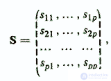
where Sij is a measure of the connection between signs xi and xj.
There are a large number of measures of communication between the signs. They differ in both the amount of computation and the aspects of communication that they reflect. Different authors propose different grounds for the classification of these communication measures (for example, Eliseev I. I. et al., 1977; Mirkin B. G., 1980; Nikiforov A. M. et al., 1988). There will be considered two representative groups of relationships between the signs / Statistical methods ..., 1979 /.
In the first group, the principle of covariance is used, and in the second, the principle of conjugacy of characters. Based on the first principle, the conclusion about the existence of a relationship between variables is made when an increase in the value of one variable is accompanied by a steady increase or decrease in the values of another. In mathematical expression, the task is reduced to the calculation of the covariance, that is, the concomitant change in the numerical values of the characteristics. This primarily relates to the Pearson correlation coefficient (r kj ), which is a product of moments and is a measure of the linear relationship between two variables xk and xj. It is calculated by the formula
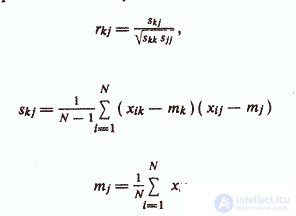
Many measures of communication differ from the reduced Pearson correlation coefficient in the external form, but are, in fact, an algebraic transformation of this coefficient, taking into account the specificity (type) of the compared features. For example, the Spearman's rank correlation coefficient (rs), often used to analyze ordinal variables, is an algebraic simplification of rkj. The same can be said about the point bisterial correlation coefficient (rpb) which serves as a measure of the relationship between dichotomous and quantitative variables. Some other coefficients, in particular, the tetrachoric correlation coefficient (rtet) and the bisterial correlation coefficient (rbis), can be interpreted as approximations of rkj for certain types of features / J. Glaus et al., 1976 /.
A somewhat different approach in the considered group of communication measures is based on counting the number of discrepancies in the ranking of objects by matching variables. This approach was developed by M. Kendall (1974), when he attempted to interpret the process of measuring the relationship between variables without resorting to the principle of the production of moments. He considered two ordinal signs xi and xj, for each of which N objects are displayed in N consecutive ranks (1, 2, ..., N). Of N objects, N (N - l) / 2 pairs are formed, and for each pair, the number of coincidences of the order on the xj sign with the order on the xj sign is calculated. This amount is denoted by "P". In the same way, the number of “Q” mismatches (inversions) is determined.
The rank correlation coefficient, called Kendall's Tau, is calculated using the formula
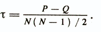
Despite the differences in approaches, there is a close logical connection between the Spearman’s and Kendall’s rank correlation coefficients, as noted in (G. Glass et al., 1976). At the same time, Kendall’s τ has an interesting interpretation for mathematical statisticians: if two objects are randomly selected from N objects, then the difference between the probability that they will have the same order both in xi and xj, and the probability that they have there will be a difference in orders in xi and xj, equal to τ ("tau"). Based on the count of the number of matches and inversions, a number of different communication measures have been constructed. In particular, this principle is used in the coefficient of Kerten and Glass (rrb) bead rank correlation, which is used to study the interaction of dichotomous and ordinal variables. At the same time, Glass / Glass GV, 1966 / showed that rrb is similar to the bisterial correlation coefficient for ordinal variables and for its calculation it is possible to do without counting matches and inversions.
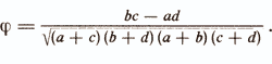
The second extensive group of communication measures, based on the principle of mutual contingency, aims to clarify the following fact: do some values of one attribute appear simultaneously with specific values of another more often than can be explained by an accidental coincidence of circumstances. In this case, only the fact of the presence or absence of the characteristic values of interest is recorded, regardless of their quantitative expression / Nikiforov AM et al., 1988 /. A common, as it were, transitional factor for the first and second groups of communication measures is the coefficient φ that is popular in psychodiagnostic studies, which is designed to measure the connection between two dichotomous features or, in other words, to analyze contingency tables 2X2 (Table 2).
Table 2. Contingency table of dichotomous features
| Sign xj | Symptom xi | Total | |
| 0 | one | ||
| one | but | b | a + b |
| 0 | with | d | c + d |
| Total | a + c | b + d | |
The coefficient φ is an algebraic simplification of the usual Pearson correlation coefficient rij taking into account the specifics of dichotomous features and is calculated by the formula
Other measures of communication based on the principle of mutual conjugacy, for example, the coefficients of Chuprov, Kramer, the Pearson contingent, etc., are discussed in detail in / Kendall, M., et al., 1976; Mirkin B. G., 1976; Eliseeva I. I. et al., 1977; Statistical methods ..., 1979; Ayvazyan S. A. et al., 1983 /.
Table 3. Recommended measures of communication between different types of signs
Open the table »» »
In general, on the problem of choosing one or another measure of communication for solving a specific task, the following can be said. The application to the same data of different communication measures often leads to different results. This is due to the fact that the mathematicians who constructed the correlation coefficients, as a rule, investigated their properties in extreme situations - about 0 or 1 / Eliseeva I. I. et al., 1977 /. The behavior of various communication measures within the [0,1] interval is relatively little studied. Therefore, in practice, the preferred choice of a measure of communication can be difficult to justify, and the results of using different measures are difficult to compare.In many ways, this choice is determined by the personal sympathies of the researcher. As a recommendation, table 3 is proposed, which summarizes the most frequently used linkage measures in psychology for different types of signs. In detail, all the coefficients listed in the table are analyzed in / Jasc J. et al., 1976 /.
The matrix of proximity (remoteness) defines the relation "object-object" and is a square symmetric matrix NxN with non-negative elements
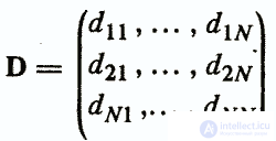
The elements dij are values of some measure of proximity (distance) between objects xi and xj. Most often, data analysis uses distance measures. These measures include the following requirements:
1. The maximum similarity of the object with itself -
2. The requirement of symmetry -
3. Fulfillment of triangle inequality -
Последнее требование предъявляется к матрицам расстояний (диагональные элементы должны быть равны нулю). Матрица D , удовлетворяющая перечисленным трем требованиям, допускает толкование структуры взаимоотношений объектов исследования как некоторой геометрической конфигурации точек в многомерном пространстве признаков.
Приведем наиболее распространенные меры расстояния между объектами хi и хj
.
1) Евклидово расстояние -
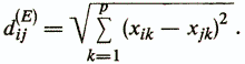
This measure can be used to calculate the distance between objects described by quantitative, qualitative, and dichotomous features. Its use is advisable when the signs are uniform in meaning and equally important for the problem being solved.
2) Weighted Euclidean distance -
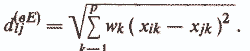
This measure is used when it is necessary to quantify the importance of any signs or to equalize the masses of heterogeneous signs.
3) Mahalanobis Distance -
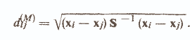
de S is the covariance matrix of the general population, from which the objects xi and xj are extracted
. Its elements are calculated by the formula Ski (see above). This measure is applied when there is a strong dependence and non-uniformity of the studied features, since it is invariant to linear transformations of the feature space (changing the scale and rotation of the axes).
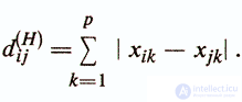
4) Minkowski distance -
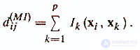
This distance is also called the “urban metric”, since in this case the distance between points is determined similarly to the distance along mutually perpendicular streets of city blocks / V. V. Aleksandrov and others, 1990 /. A city metric is used to measure the distance between objects described by ordinal features. I k (xi, xj
) is equal to the difference of the numbers of gradations according to the k-th attribute of the compared objects xi and xj
.
5) Hamming distance -
This measure is most often used to determine differences between objects defined by dichotomous features and is interpreted as the number of character values mismatch between the considered objects xi and xj
. For dichotomous features, it corresponds to the square of the Euclidean distance. As for the Euclidean distance, weighted Hamming distance can be used.
6) Other proximity measures for dichotomous features.
These proximity measures are usually based on counting the number of zero or single component features that match or are not matched on objects xi and xj.
and giving this number varying degrees of importance. These measures are discussed in detail in / Bonner, R. E., 1969; Zhitkov G. N., 1970; Eliseeva I. I. et al., 1977 /.
Presentation of information about the structure of experimental data by means of matrixes of connections of signs S and proximity (remoteness) of objects D serves as an intermediate link in the process of building diagnostic models y = y (x) of various types. Regardless of this type, there are two main strategies for determining the parameters of diagnostic models. The first strategy uses methods that directly rely only on the particular configuration of the experimental data structure that has been formed, which finds its expression in numerical relations of similarities and differences in TED elements. Therefore, it is called a strategy based on the autoinformative criterion of experimental data . For example, if a group of strongly correlated features is found in the matrix of connections S , then perhaps this is a consequence of the reflection of the signs included in the group of an empirical factor corresponding to the required diagnostic construct. Or, for example, if, based on the analysis of the components of the matrix of distances D , it is possible to establish that the distribution of objects in the feature space consists of several geometric groupings, then this may be a reason to try to explain this fact by the differences of the objects under study on the property being tested and build an adequate diagnostic algorithm. .
At the same time, it is necessary to be well aware that the revealed groupings of objects to a large extent depend on the type of measure used between the objects and on the system of features used. So, in particular, the “good” geometrical structure of the distribution of objects in any subspace of features, from the point of view of the diagnostic problem being solved, can be “ruined” by adding “noisy” features to this subspace or “suppressed” by a more “strong” structure that reflects the irrelevant property factor. In turn, significant relationships between signs can be formed due to stratification of a sample of objects under the influence of an extraneous factor. Conversely, the lack of correlation may be explained by the effect of unaccounted sample characteristics (for example, for individuals of different sexes, the signs of correlation may be high, but they may have opposite signs. Therefore, in a mixed sample, the correlations of the same signs will be close to zero).
The examples given, as well as other examples considered in the following sections, show that it is often necessary to use additional information to build a diagnostic model, besides that directly contained in the original TED. This additional information is called training, and it carries information about the empirical relationship between the objects of research obtained in one way or another. Training information is formed on the so-called criteria of external information content, or, in other words, external criteria . This information is presented in various forms. This can be a binding to the objects of the values of the “dependent” variable measured in the quantitative scale, the number of the class that is homogeneous by the property being tested, the sequence number (rank) of the object xi>
in the series of all objects, ordered by the degree of manifestation of the diagnosed property, and, finally, the totality of values of a set of external (not included in the analyzed TED) signs that characterize the psychological phenomenon being tested. When using training information, objects in the original space of signs in accordance with an external criterion seem to be “painted in various colors,” which makes it possible to more purposefully find ways of transforming the original signs into the resulting diagnostic indicator. Methods based on the application of external criteria constitute the second strategy for determining the parameters of diagnostic models.
Depending on the coincidence of the autoinformative criteria with the external informative criteria, the methods of the first and second strategies can lead to similar results. At the same time, these results largely depend on which transformations reveal the information potential of the initial experimental data. There is no diagnostic "informativeness at all." Informational content of data exists only in relation to the type of diagnostic model used, the choice of which, in turn, is determined by technical resources and theoretical ideas of specific researchers.
In psychodiagnostics, linear models prevail, in which the resulting indicator is represented as a weighted sum of the initial features.
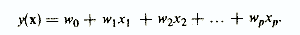
The prevalence of linear models is primarily due to their greatest simplicity, clarity and "workability", which allows, in particular, to manually process the test results. For example, a laboratory technician participating in a psychodiagnostic experiment compares the subject's answers to test questions with a special “key”, sums the coincidences with certain weights and thereby implements a linear diagnostic model.
From a mathematical point of view, the development of diagnostics occurs in the direction of abandoning linear models / Ayvazyan S. A. et al., 1989 /. But, undoubtedly, they will always be of great practical importance due to their brevity and good interpretability.
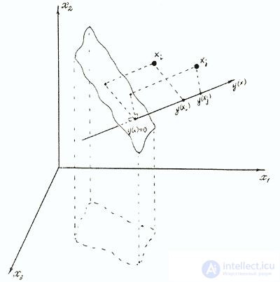
Linear models are convenient for considering geometric illustrations of the calculation of the resulting indicator. The equation y (x) = 0 is the equation of the hyperplane in the feature space (Fig.), And the distance from the object xi, which is represented by a point in this space, to the hyperplane is 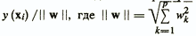 - the norm of the weight vector w.
In fig. shows two objects xi and xj and a piece of the plane y (x) = 0 in three-dimensional space. Since in this case the norm of the weight vector is chosen arbitrarily and equal to 1, the distances from xi and xj to the plane directly correspond to the values of y (xi) and y (xj). These values are often conveniently interpreted as projections xi and xj.
on any straight line in the considered feature space, perpendicular to the plane y (x) = 0 This straight line is indicated in the figure y (x).
The point of its intersection with the plane gives the value of zero on the line. Further similar geometric illustrations will be used repeatedly. This will be appropriate even when the norm of the weight vector is not equal to one, since the distortion of the scale, which is observed in this case, will not entail a distortion of the main thing - the relative position of the projections of points on the line.
Fig. Illustration of linear diagnostic feature space of a model in a three-dimensional feature space.
Depending on the angle of view, under which the linear diagnostic model is considered, it may have different names. If, for example, “y” is treated as a “dependent” variable for which a functional relationship is sought with “independent” variables (attributes) xi, then the linear model equation y (x) is called a linear regression function or a multiple regression equation. If the problem of classifying objects is considered, then y = y (x) is usually called a linear decisive function, and the equation y (x) = 0 is called the dividing boundary or the equation of the dividing hyperplane. Below, when discussing this or that method of determining the parameters of a linear diagnostic model, different terms will also be used, but, as mentioned above, a global attribute for distinguishing between these methods is whether or not the external information content criterion is involved.
Formal algorithms of the considered group of methods do not directly operate with training information about the required value of the variable being diagnosed. At the same time, this information in an implicit form is always present in the experimental data. It is laid at the very first stage of constructing a psychodiagnostic test, when the experimenter forms an initial set of features, each of which, in his opinion, should reflect certain aspects of the property under test. In this case, the reflection of this property by a separate sign, as a rule, is understood as the simplest type of connection of a sign with a diagnosed indicator - correlation xi with у. If the property being tested is homogeneous, then there is every reason to believe that the measure of information content for the final selection of signs can be the degree of coordinated action of these signs in the right direction.
Internal consistency of test assignments is an important category of methods based on the criterion of autoinformativeness of the feature system. The consistency of measurable responses of test subjects to test stimuli means that they must have a statistical focus on the expression of the general, main trend of the test. The geometrical structure of the experimental data, formed under the influence of the cumulative effect of a consistent interaction of features, in a somewhat idealized form looks like a cloud of points in the feature space that fits into the hyperellipsoid. All pairs of features with such a structure have statistically significant correlations, and the equation of the main axis of the hyperellipsoid is a linear diagnostic model of the property under test.
Practically all methods of constructing psychodiagnostic tests based on the criterion of autoinformativeness of the feature system and using the category of internal consistency of test tasks are based on the presented representations. Below will be discussed the main methods of this group.
The principal component method (CIM) was proposed by Pearson in 1901 and then reopened and developed in detail by Hotteling / 1933 /. A large amount of research is devoted to it, and it is widely represented in literary sources, referring to which you can get information about the method of principal components with varying degrees of detail and mathematical rigor (for example, Ayvazyan S. A. et al., 1974, 1983, 1989). This section does not aim to achieve a detailed presentation of all the features of the CIM. We concentrate on the main phenomena of the main component method.
The principal component method makes the transition to the new coordinate system y1, ..., ur in the original feature space x1, ..., xp which is a system of ornormalized linear combinations
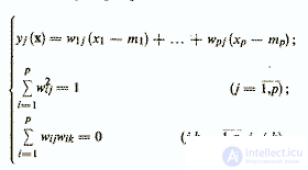
where mi is the mathematical expectation of the sign xi. Linear combinations are chosen in such a way that among all possible linear normalized combinations of the original features, the first main component of y1 (x) has the greatest variance. Geometrically, it looks like the orientation of the new coordinate axis y1 along the direction of the greatest elongation of the ellipsoid of dispersion of the objects of the studied sample in the feature space x1, ..., xp. The second principal component has the largest variance among all the remaining linear transformations uncorrelated with the first principal component. It is interpreted as the direction of the greatest elongation of the ellipsoid of dispersion, perpendicular to the first principal component. The following main components are determined by a similar scheme.
The calculation of the coefficients of the main components wij is based on the fact that the vectors wi = (w11, ..., wpl) ', ..., wp = (w1p, ..., wpp)' are eigen (characteristic) vectors of the correlation matrix S In turn, the corresponding eigenvalues of this matrix are equal to the variances of the projections of the set of objects on the axes of the principal components.
Algorithms that ensure the implementation of the principal component method are included in almost all statistical software packages.
In the method of principal components described above, the criterion for autoinformativeness of a feature space implies that valuable diagnostic information can be reflected in a linear model that corresponds to a new coordinate axis in a given space with the maximum variance of the distribution of projections of the objects under study. This approach is productive when the obvious majority of tasks of the “draft” version of the test consistently “work” on the manifestation of the property under test and suppress the influence of irrelevant factors on the distribution of objects. Also, a positive result will be obtained with a relatively small volume of a group of related informative features, but with uncoordinated interaction of extraneous factors, under the influence of which the dispersion ellipsoid homogeneity is not disturbed, but only the elongation of distribution of objects along the direction of the diagnosed trend decreases. In contrast to the principal component method, factor analysis is not based on the dispersion criterion of the autoinformativeness of a feature system, but is focused on explaining the correlations between features. Therefore, factor analysis is used in more complex cases of joint manifestation on the structure of experimental data of the tested and irrelevant properties of objects comparable in the degree of internal consistency, as well as to select a group of diagnostic indicators from the general initial set of features.
The basic model of factor analysis is written by the following system of equalities / V. Nalimov, 1971 /
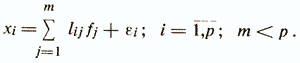
That is, it is assumed that the values of each attribute xi can be expressed by a weighted sum of latent variables (simple factors) fi, the number of which is less than the number of source characteristics, and the residual term εi with dispersion σ2 (εi) acting only on xi, which is called a specific factor. The coefficients lij are called the load of the i-th variable on the j-th factor or the load of the j-th factor on the i-th variable. In the simplest model of factor analysis, it is considered that the factors fj are mutually independent and their variances are equal to unity, and the random variables εi are also independent of each other and of any factor fj. The maximum possible number of factors m for a given number of signs of p is determined by the inequality
(p + m) <(p - m) 2,
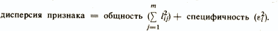
which must be performed so that the task does not degenerate into a trivial one. Данное неравенство получается на основании подсчета степеней свободы, имеющихся в задаче /Лоули Д. и др., 1967/. Сумму квадратов нагрузок в формуле основной модели факторного анализа называют общностью соответствующего признака xi и чем больше это значение, тем лучше описывается признак xi выделенными факторами fj. Общность есть часть дисперсии признака, которую объясняют факторы. В свою очередь, ε2i показывает, какая часть дисперсии исходного признака остается необъясненной при используемом наборе факторов и данную величину называют специфичностью признака. In this way,
Основное соотношение факторного анализа показывает, что коэффициент корреляции любых двух признаков xi и хj можно выразить суммой произведения нагрузок некоррелированных факторов

Задачу факторного анализа нельзя решить однозначно. Равенства основной модели факторного анализа не поддаются непосредственной проверке, так как р исходных признаков задается через (р+m) других переменных — простых и специфических факторов. Поэтому представление корреляционной матрицы факторами, как говорят, ее факторизацию, можно произвести бесконечно большим числом способов. Если удалось произвести факторизацию корреляционной матрицы с помощью некоторой матрицы факторных нагрузок F , то любое линейное ортогональное преобразование F (ортогональное вращение) приведет к такой же факторизации /Налимов В. В., 1971/.
Существующие программы вычисления нагрузок начинают работать с m =1 (однофакторная модель) /Александров В. В. и др., 1990/. Затем проверяется, насколько корреляционная матрица, восстановленная по однофакторной модели в соответствии с основным соотношением факторного анализа, отличается от корреляционной матрицы исходных данных. Если однофакторная модель признается неудовлетворительной, то испытывается модель с m=2 и т. д. до тех пор, пока при некотором m не будет достигнута адекватность или число факторов в модели не превысит максимально допустимое. В последнем случае говорят, что адекватной модели факторного анализа не существует. Если факторная модель существует, то производится вращение полученной системы общих факторов, так как значения факторных нагрузок и нагрузок на факторы есть лишь одно из возможных решений основной модели. Вращение факторов может производиться разными способами. Наиболее часто это вращение осуществляется таким образом, чтобы как можно большее число факторных нагрузок стало нулями и каждый фактор по возможности описывал группу сильно коррелированных признаков. Также можно вращать факторы до тех пор, пока не получатся результаты, поддающиеся содержательной интерпретации. Можно, например, потребовать, чтобы один фактор был нагружен преимущественно признаками одного типа, а другой — признаками другого типа. Или, скажем, можно потребовать, чтобы исчезли какие-то трудно интерпретируемые нагрузки с отрицательными знаками. Нередко исследователи идут дальше и рассматривают прямоугольную систему факторов как частный случай косоугольной, то есть ради содержания жертвуют условием некоррелированности факторов.
В завершение всей процедуры факторного анализа с помощью математических преобразований выражают факторы fj через исходные признаки, то есть получают в явном виде параметры линейной диагностической модели.
There are a large number of methods of factor analysis (rotations, maximum likelihood, etc.). Often, several versions of such
продолжение следует...
Часть 1 Designing psychodiagnostic tests: traditional mathematical models and algorithms
Часть 2 Contrast group method - Designing psychodiagnostic tests: traditional mathematical models
Часть 3 6. Standardization and testing of diagnostic models - Designing psychodiagnostic
Часть 4 - Designing psychodiagnostic tests: traditional mathematical models and algorithms

Comments
To leave a comment
Mathematical Methods in Psychology
Terms: Mathematical Methods in Psychology