Lecture
In many areas of practical psychology, measuring psychodiagnostic methods are widely used, which include tests for measuring abilities, achievements, and instrumental methods based on standardized self-report - questionnaires and subjective scaling techniques. The correctness in the application of these techniques is ensured not only by meaningful ideas, but also by meeting the special requirements of psychometrics - the requirements of validity, reliability, and representativeness of test norms.
Test methods are designed to solve a certain limited range of tasks. These are the tasks of mass express diagnostics. Here errors are not excluded in individual cases, the diagnosis and prognosis are given only with probabilistic accuracy.
This report describes specific techniques of empirical-statistical debugging tests that a psychologist can use both in the presence of modern computing equipment, and in its absence. These techniques allow you to check whether the test “works” as a whole and, if it poorly differentiates the subjects, in which parts (tasks, questions) the test “does not work”. The use of these techniques is useful and necessary not only in the development of new tests, but also with any change in the diagnostic situation in the application of the old test (for example, the transition from voluntary to compulsory examination), when transferring the test from one population (on which test standards are established) to another . This primarily refers to the techniques of self-report and, in particular, to test questionnaires, which depend entirely on how a particular subject interprets the semantics of the questions and links it to the subjective hypothesis about the purpose of the survey. But the algorithms described here are applicable to any other tests: the results of the test tasks can also be formally encoded as a binary variable - 1 (“decided”) or 0 (“not decided”).
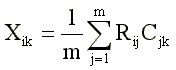
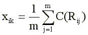
The test questionnaire consists, as a rule, of so-called whether questions or yes-no questions [4]: each question contains a statement with which the subject is asked to agree or disagree. As a result, the response of the subject is encoded as a dichotomous variable with the values “+1” (“true”) and “-1” (“incorrect”). The test score is calculated by summing the answers “true” to the “direct” test items (these are questions positively related to the measured feature) and the answers “incorrectly” to the “reverse” items (questions negatively related to the measuring feature). Algebraically, this simplest method of calculating a test score can be described by formula (1):
Where:
Hik - the score of the i-th test on the k-th scale (line);
Rij is the answer of the i-th test subject to the j-th item of the test questionnaire;
Cjk is the key (scale value) of the jth item on the kth scale;
m is the number of points in the k-scale (for which Cjk is No. 0).
Usually Rij = {-1, + 1} and Cjk = {- 1, 0, +1}.
In order to somehow minimize the already large errors of the test questionnaire, the psychologist must understand the psychological meaning of this procedure. The test questionnaire item should be an empirical indicator of the diagnostic concept - a personality trait. If a psychologist comes to a small town, in which all residents take a step to the station, then the question “Do you order a taxi before heading to the station?” Here will obviously have nothing to do with such features as “anxiety”. In such circumstances, such a question is simply incorrect, not informative, it should be excluded from the list. Before applying a test questionnaire on a special contingent of persons, the psychologist should try to look at each question through the eyes of the subject. This requires considerable professional intuition. In the presence of a large battery of questions, no psychologist can manage to fully imitate the answers of the subjects. Here, an empirical-statistical analysis of items comes to the rescue (a special term “item analysis” has been established in foreign testimony) [7].
At present, no serious attempt to construct or adapt tests can do without the use of this apparatus.
Apparatus empirical and statistical analysis of items opens up the possibility for adapting the methodology to the specific conditions of its application. This feature consists of modifying the scale keys for individual items (Cjk values). The usual archaic measurement strategy of such a device is that the psychologist reformulates the question itself. For example, instead of asking about ordering a taxi in a small town, he will ask the question “Do you arrive at the station half an hour before the train departs?” Thus, the list of questions changes. The results obtained from respondents from large and small cities are incomparable. The opposite tactic is to leave the list of questions unchanged, but in different cases use different scale vector vectors <С>. (In all cases, both questions are asked. This approach allows us to combine two (usually regarded as independent) test design tasks: selection of informative features (items from Cjk No. 0) and the construction of a scale (refinement of the gradual Cjk).) Сjk = 0.0 in a small town (where k is the scale of anxiety) and, conversely, Сjk = +1.0 in a large one.
How can one empirically determine the Cjk values in the absence of a computer, i.e. manually? Here we describe the simplest method, which, as shown by studies specially carried out by us, gives results that coincide quite well with the results of cumbersome computer algorithms.
The ideas of this algorithm in various modifications were used in a variety of works by foreign and domestic authors. Consider a situation arising in the absence of an external criterion of validity.
Let the psychologist have a test questionnaire focused on the measurement of a single personality trait (one-dimensional questionnaire) and containing M questions. The psychologist does not have any a priori empirical information about the surveyed contingent, but proceeds from the assumption that the individuals in this sample differ significantly from each other in the degree of manifestation of the trait under consideration k. The psychologist wants to adapt the test questionnaire to measure the k trait on this contingent by specifying the Cjk scale keys. For this, it is advisable for him to take for a preliminary psychometric study a random sample of N individuals. For successful analysis of items, it is required to use M і 50 and N і 100. Smaller values of M and N, as a rule, lead to too large dropouts of points (many potentially informative, diagnostically valuable points get Cjk = 0).
On the sample, the psychologist conducts a survey and gets an array of results in the form of a rectangular matrix of N × M, where the subjects are in rows, points in columns, and Rija values of answers of the i-th subject to the j-th question of the test questionnaire at the intersection.
For each column (for each item), the psychologist, based on the initial assumptions, assigns С0jk — initial scale keys. Then, for each row (of each subject) of the matrix | R | formula (1) is calculated total test score Hik. Among all {X}, 30% of subjects with the highest test score and 30% with the lowest are searched. They are included respectively in the "high" and "low" extreme groups. In the future, for each item, only answers from subjects from extreme groups are taken into account. The Cjk scale keys are refined by calculating the four-cell correlation between the responses to the item and entering the extreme group. For each item, a 2 × 2 contingency matrix is constructed:
| Extreme group | ||
| Answer | High | Low |
| "Right" | a | b |
| "Wrong" | c | d |
The 2 × 2 signs indicate the frequencies. For example, in cell a, the frequency of occurrence of those subjects who fall into the “high” group and answered “true” to this j-th item of the questionnaire is summed up; in cell b - the number of subjects from the “low” group who answered “true”. etc. It is obvious that a “good” item, which is highly discriminative with respect to extreme groups, should have a high contrast of values a and b , on the one hand, and at the same time high contrast with and d on the other. At the same time, the contrasts should have the opposite sign: if a is greater than b (the “high” group most often answers “true”), then c should be less than a (the “low” group most often answers incorrectly); on the contrary, in the case of “inverse” points, when the difference a – b is negative, then the difference c – d must be positive. There are various factors that take into account these requirements [6], [3]. We propose to use the most popular of them fi-coefficient [27]:
(2)
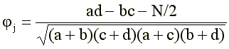
where N is the sum of all the elements of the plate: N = a + b + c + d (In the case of “reverse” points, when the difference (ad-be) is negative, the value must be added to the numerator, on the contrary, the numerator (2) gets the form: ad-bc + N * / 2.)
Since the use of equal and well-known in terms of extremal groups a + c = b + d = S, formula (2) is somewhat simplified:
(3)
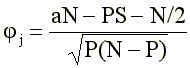
where P is the sum of answers “right” for this item: P = a + b.
The significance of the phi-coefficient is determined from the following approximate relationship:
(four)
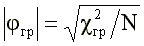
where: c2gp is the standard quantile of the chi-square distribution with one degree of freedom. As known. c21; 0.05 = 3.84 and c21; 0.01 = 6.63.
Thus, if at sampling N = 100 the calculated value of the fi-coefficient exceeds modulo 0.26, then this means that with a negligible error probability of 1%, it can be concluded that this item makes a significant contribution to the total score. If j і 0.26, the item should be considered “direct” (the answer is “true” testifies in favor of the measured feature), if j Ј -0.26, the item should be considered inverse (the answer “incorrectly” indicates the benefit of the measurement feature).
If the number of points M = 50, the psychologist will have to build 50 matrices of 2 × 2 and 50 times to calculate the phi coefficient using formula (3). It is clear that in order to facilitate the procedure, a pocket calculator should be used when calculating formula (3), and for constructing contingency plates it is convenient to make a stencil (like a key when calculating total points): on a strip of transparent paper (polyethylene), indicate the arrangement of rows on the rows of the matrix | R | subjects from the "high" group and triangles - subjects from the "low" group. Then, if a “+” in a column gets in the circle, the unit is written in the “a” cell, if the “+” in the triangle hits - in the “b” cell, etc.
After jj has been calculated for all M points and checked for significance (j is compared with | jgr |), the psychologist derives new refined values of C1jk: if jj i jgr, then C1jk = +1; if jj Ј -jgr, then C1jk = -1, if -jgr <jj <jgr, then C1jk = 0 (i.e., the item is not taken into account when calculating the total score).
If all the refined C1jk coincided with the original proposed keys C0jk, then we can conclude that the psychometric experiment fully confirmed the tested test questionnaire for all items of which it consists. But in practice, such a complete coincidence never happens.
In the absence of a full match, a new computational processing cycle is required. According to the specified vector - key <С1> by the formula (1) the total points for all subjects are calculated again. Then again, extreme groups are determined, and the fi-correlations for all M points of the questionnaire are again calculated. (If several subjects at the border between an extreme and a neutral group got the same score at once, then all subjects with the same score should be included in one group, ensuring that the extreme was closer to 30%, then the number of extreme groups may not be the same and the formula should be used (2) when calculating jj.) Obviously, the procedure reaches the effective stop if <Ct> = <Ct + 1>, that is, when the key obtained at the next processing step coincides completely (over all j) with the key obtained on the previous sha e.
In this case, this moment can be determined in advance: the desired condition is reached already when the compositions of the “high” and “low” groups are stabilized (namely, the compositions of the extremal groups determine the values of the fi-correlation). To assess the quality of items, a more time-consuming computationally point-biserial correlation is often used [2], [25]. In this case, you can stop with the equality ct + 1ik = ctik
We have accumulated significant empirical experience in using this simple algorithm. With the help of this algorithm, students of general and special workshops of the Faculty of Psychology master the techniques of analyzing items [22]. Comparison of the results of this algorithm with more accurate computer algorithms (for example, factor analysis by the principal component method) showed that satisfactory correspondence of “manual” and “computer” keys is achieved on average already at the fifth or sixth approximation step.
It must be said that the convergence (stabilization rate of the vector <Сtjk>) of this algorithm depends on the degree of elaboration of the questionnaire itself. This algorithm quickly leads to the selection of stably useful items if most of the items in the questionnaire are good. On the contrary, if such items are less than half, then the procedure is delayed. In this case, it is better to stop the calculation process already after the first approximation of <С '> and, if too few significant jj are found, to reformulate old or add new questions (then conduct a new survey).
Significant indicators jj indicate the consistency of this item with the diagnostic concept of the entire questionnaire as a whole - with most of the other items. A. Anastasi refers the considered indicator to internal validity [2]. This is to some extent justified if different expert psychologists were involved in the formulation of points. The fact that correlations were found between the answers to different points indicates the convergent validity of the points as a kind of microtest. But with too high correlations, an increase in single-stage reliability (the Cronbach alpha coefficient, see [23]) is combined with a decrease in external validity — validity by external criterion.
When selecting items by the external criterion (when building a test by criterion), the described simple computational techniques can also be applied. So, for example, we want to build or adapt a questionnaire of motivation of professional achievements to the prediction of academic performance of university students. An acceptable strategy is as follows. By the criterion of academic performance (external criterion), extremal groups of students who are obviously successful and unsuccessful are selected. These two groups make up the sample that presents the test questionnaire. Then on the matrix | R | the fi-correlation of each item is calculated with a hit in the “high” or “low” group by the external criterion (the numerator in formula (2) takes the form: (ad-bc).). On the basis of significant j, the key values Cj are determined, which is then used to calculate the prognostic performance score based on the survey results. (With a more correct prospective validation, the moment of selection of extreme groups is done after the survey itself. This requires the involvement of large samples - “with a margin” - to isolate extreme groups.) Yu.M. applied a similar strategy (using the cosine-pi coefficient). Orlov during the construction of the questionnaire "motivation of achievement" [17].
Unfortunately, the selection of items according to the criterion rarely fulfills the obligatory rule of “cross validation” [2]: the obtained values of jj must be checked on an independent sample (or on half of the whole sample). It is also rarely taken into account, unfortunately, that building a test by criterion is a pragmatic strategy that does not ensure the psychological homogeneity of the measured construct: psychologically different factors can be included in the <С> key. Test questionnaires based on external criteria, with subsequent factorization, as a rule, “break up” into a number of independent factors. From this point of view, the optimal test battery (set of points) by the criterion can be obtained by applying the analysis of multiple correlations: the weights bj for each point in the multiple regression equation are “cleared” from the unjustified (from the point of view of economy) duplication of points too closely correlated with each other with a friend (for the algorithm, see [1], [26]). But the computational complexity of this method requires the mandatory use of a computer, already when M> 5.
In those cases when we want not only to predict, but also to know with what psychological factors the prognosis is provided, we must carry out internal validation of the test questionnaire.The described algorithm for calculating j for consistency with the total score retains its meaning.
За период с 1977 по 1984 г. с помощью алгоритмов подобного типа нами проведен анализ пунктов при адаптации и конструировании многих личностных опросников: на измерение тревожности, импульсивности, догматизма, локуса-контроля [12], социальной желательности, склонности к риску, конформности, экстраверсии — интроверсии, по Айзенку, нейротизма, по Айзенку, самоуверенности, завистливости (неопубликованные материалы практикумов по психологии) и др. В учебном пособии [21] предлагается практическое задание для овладения этой процедурой на материале опросника ригидности. Эта же процедура применима для экспериментальной отладки опросниковых шкал установок и отношений, как, например, «удовлетворенность браком» [18], «отношение к стрессу» (неопубликованные материалы ВКНЦ АМН СССР), «отношение к психометрике» (неопубликованные материалы спецсеминара по психометрике).
Укажем пример результатов работы этого алгоритма на материале известного опросника Айзенка. Как известно, этот опросник включает сразу три шкалы, так что для каждого пункта по аналогичному принципу могут быть рассчитаны jik по отношению к попаданию в экстремальную группу по любой из трех шкал (при любом k). Например, вопрос «Часто ли вы действуете под влиянием минутного настроения?» Вместо полюса «экстраверсия» оказался эмпирически отнесенным к полюсу «нейротизм» (испытуемые интерпретируют такое поведение, как выражение «эмоциональной неустойчивости», а не как выражение «самоуверенной импульсивности», свойственной экстравертам). Вопрос «Когда на вас кричат, вы отвечаете тем же?» вместо полюса «экстраверсия» оказался скоррелированным с попаданием в группу «откровенных» («верно» значимо чаще отвечают те, кто набирает меньше очков по шкале «лжи»). Легко видеть, что подобные нюансы смысловой интерпретации вопросов трудно предвидеть, не располагая эмпирическими данными и не проводя их статистической обработки.
Если первый из описанных здесь алгоритмов является традиционным (для мировой психометрики) способом анализа пунктов, пригодным для ручных вычислений, то данный алгоритм — наша авторская разработка. Его преимущества — в еще большей простоте вычислений, более быстрой и более высокой дифференцирующей силе построенной шкалы.
При том же уровне структурированности массива |R| сходимость ключей достигается за счет 3-4 итераций (апробировано на ЭВМ с помощью программ, составленных на языках Бейсик и Фортран А.Г. Шмелевым). Выделенный вектор опять же высоко конгруэнтен (совпадает) с первой или второй главной компонентой одномерного опросника. При факторизации одномерного опросника практически всегда выделяются два фактора: один соответствует измеряемому свойству, другой — социальной желательности ответа; сила второго фактора зависит от диагностической ситуации и уровня подозрительности контингента испытуемых.
Алгоритм раздельного коррелирования ответов, подобно очень сложным алгоритмам латентно-структурного анализа [14], позволяет учитывать при подсчете суммарного балла с разным весом ответы «верно» и «неверно». Формула (1) несколько модифицируется:
(five)
где C(Rij) — ключ, заданный как вторичная переменная, принимающая различные значения в зависимости от того, какое из заранее предусмотренных значений Rij реализовано. Такая модификация позволяет учесть разную силу ответов «верно» и «неверно», их разное диагностическое значение.
На каждом очередном t-м шаге вычислений по ключу <Ct-1ik> и по матрице |R| с помощью формулы (5) подсчитываются суммарные баллы xik. Как и в первом алгоритме, из {x+} выделяются «высокая» и «низкая» группы, и для каждого j-го пункта строится четырехклеточная табличка сопряженности. Ключ для ответа «верно» определяется по формуле:
(6)
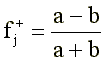
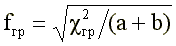
Понятно, что f+j достигает +1, если «верно» отвечают только представители «высокой» группы, и -1, если «верно» отвечают только испытуемые из «низкой» группы. Значимость f+j можно оценить с помощью следующего приближенного соотношения:
(7)
The key for the answer "incorrectly" is determined by the formula:
(eight)

The test of the significance of fj is similar, taking into account the substitution c + d = a + b.
In the computer version, it is easy to use keys that take all possible values on the interval [-1, +1], i.e. equate C (Rjk) = fjk. For manual calculations, it is better to use the seven-point integer scale [-3, +3] with the transition formula
Cjk = 3 fjk
and rounding to the nearest integer. Of course, assigning non-zero points to Cjk is necessary only if fj significantly exceeds fgp in absolute value.
Практическое испытание данного алгоритма показало, что более высокими fj, как правило, обладают менее социально одобряемые ответы. Например, в опроснике на «склонность к риску» ответ «верно» на вопрос «Я быстро меняю свои интересы и увлечения» получил f+ = 0.60 (Р < 0.05), а ответ «неверно» получил f - = —0.26 (не значимо). Понятно, что устойчивость интересов — более социально одобряемая форма поведения, поэтому более информативен ответ «верно» (контраст между а и b сильнее контраста между c и d. По этим же причинам для вопроса «Я быстрей испытываю скуку, чем большинство людей, делающих то же самое»:
f+ = 0.63, а f - = -0.29.
Информативнее менее «благоразумные» ответы. Например, для пункта «Люди слишком часто безрассудно тратят собственное здоровье, переоценивая его запасы» f+ = -0.14, a f - = +0.75 (значимо на уровне р < 0.05). В опроснике на «тревожность» в вопросе «Я опасаюсь, что о моих недостатках станет известно другим» более информативным оказался ответ «неверно»: f+ = 0.33, a f - = -0.78.
Достоинство алгоритма-2 в том, что он позволяет отыскать значимые связи там, где алгоритм-1 фиксирует только незначимую корреляцию. Читателю можно посоветовать самому убедиться в этом, подставляя в табличку 2 × 2 различные значения частот а, b, с, d. Поэтому алгоритм-2 можно считать более эффективным и при отборе пунктов по внешнему критерию. Не требуя вычисления никаких подкоренных выражений, алгоритм-2 может быть реализован даже в отсутствии карманных калькуляторов и таблиц. (Оценку значимости можно производить по формуле c2эм = f2(a + b) и сравнивать c2эм и c2гр.)
Обсуждение компьютерных алгоритмов нельзя не начать с факторного анализа. Вот уже более полувека факторный анализ остается основным инструментом психометрики индивидуальных различий. Следует различать применение факторного анализа для обоснования теоретических представлений (о структуре личности, структуре интеллекта) и его применения для проверки надежности и валидности методик. Факторный анализ особенно необходим в тех случаях, когда психолог имеет дело с многомерным (многофакторным) тестом и хочет получить «простую» факторную структуру, т. е. такую, в которой максимальное количество пунктов получит значимые нагрузки (значения Сik) только по одному фактору.
Но и в случае одномерных тест-опросников не следует отказываться от возможности применить факторный анализ, если такая возможность имеется (теперь практически все вычислительные центры располагают стандартным пакетом с программой факторного анализа). Факторный анализ позволяет обеспечить дискриминантную валидность тест-опросника по отношению к артефактному фактору социальной желательности значимые Сik присваиваются только тем пунктам, которые имеют незначимые или взаимно уравновешивающие друг друга нагрузки по фактору социальной желательности [24].
Опыт применения факторного анализа к изучению эмпирических корреляции между пунктами таких популярных многофакторных (многошкальных) тестов, как 16PF и MMPI обсуждался нами подробно в другом сообщении ([10], в печ.). Отметим здесь только, что в большинстве практических ситуаций нельзя ожидать, что выборка испытуемых окажется столь репрезентативна что исчерпывающим образом будет воспроизведена вся факторная структура тест-опросника. Наоборот, чаще всего больший вес получают те факторы, которые соответствуют специфичные для данной выборки направлениям межиндивидуальных различии, а те факторы, по которым различия не найдены, вообще исчезают. В практических целях использование факторного анализа пунктов теста эффективно в такой модификации, когда в исходный прямоугольный массив |R| в качестве M+1-гo столбца в дополнение к М пунктам теста добавляется переменная -критерий (или несколько критериев). В этом случае факторный анализ позволяет одновременно увидеть и то, с какими факторами связан критерий, и то, из каких пунктов состоят эти факторы в данном случае.
Если психолог — пользователь компьютера — может заказать программу регрессионного анализа, то у него возникает удобная возможность произвести отбор оптимальной компактной батареи (перечня) пунктов по критерию: значимые регрессионные веса получают только те пункты, которые вносят свой собственный незаменимый вклад в предсказание критерия. В сочетании с факторным анализом в указанной выше модификации регрессионный анализ одновременно обеспечивает психолога пониманием тех психологических факторов (механизмов), благодаря которым достигается (или потенциально может быть достигнуто) предсказание.
Like factor analysis, cluster analysis deals with the M × M matrix of all possible pairwise correlations between all points of the questionnaire. The hierarchical clustering algorithm according to the average distance method (see [8]) groups the points into clusters, corresponding, as a rule, to the factors obtained after the varimax rotation of the main components.
Psychologists who do not have standard computer programs, it is useful to get acquainted with the book by J. Davis, which lists listings (texts) of factor, regression and cluster analysis programs in Fortran, as well as popular explanations for them, focused on subject specialists [9].
The concept of “cliques” has long been known from combinatorics: it is a complete subgraph, that is, a subset of the vertices of a whole graph, within which all possible pairs of vertices are connected by edges [13]. In our works, we prefer to use this term in the transcription "klaik", freed from the negative evaluation hue [19].
As is known, cluster analysis algorithms solve the problem of splitting objects (test points) into a set of disjoint classes. This is a pretty strong limitation that it is not necessary to apply to empirical data, since fuzzy intersecting categories (groupings of objects) may have the best conceptual interpretability. Hard partitioning breaks some groupings that lie on the boundaries between other groups. It is of research and practical interest to use in the analysis of items of large multidimensional questionnaires of the klaik-analysis algorithm, which makes it possible to extract from the intercorrelation matrix between the points, first of all, the clinker, i.e., a subset of points related to each other by means of significant correlations.
The authors of the article in the language of the translator Fortran was written and practically implemented on a computer EU-1055 and EU-1060 program, which allows you to select the main claikey from the matrix of high dimensionality. According to this program, an empirical histogram of the frequency distribution of all calculated correlation coefficients was constructed on the basis of the matrix of intercorrelations between the points. (We used the linear Pearson correlation coefficient with the preliminary normalization of correlated parameter-points.) As expected, for heterogeneous multidimensional questionnaires, this distribution turned out to be very close in shape to the normal curve. Based on this distribution, an empirically justified threshold of significant correlation was assigned, which, according to the “three sigma” rule, cuts off 0.1% of all correlations. With respect to this threshold, the computer then iterated through all the clips. At the same time, the new item was credited to the key in the event that the module of its correlations with all the other points from the key was not below the threshold G.
The program was applied to an array of data received from 380 subjects using a Kattel 16PF test questionnaire (Form B). For these data, according to the “three sigma” rule, the threshold of a deliberately nonrandom significant linear correlation turned out to be equal to 0.18.
To select the most important clips in the computer's memory, an array was reserved - the clips directory. The very first key was recorded in this array immediately. The second click was compared with the first for the following similarity coefficient:
(9)
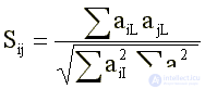
where: Sij is the coefficient of similarity (cosine) of the vectors describing the i-th and j-th clouse; aiL is the L-th element of the ith vector-clique.
Initially, aiL can take only one of the three values {-1, 0, +1), where 0 indicates the absence of the given L-th item in this i-th key, +1 means that the positive correlation between the L-m and the first non-zero value that exceeds the G peak. klaika element, -1 — a negative G correlation between the i-th and the first nonzero klaika element, which exceeds the modulus threshold G
With each new dedicated key, the program performed the following operations. The new key - candidate - was compared in order (starting from the first) with all the clips included in the catalog. If none of the clips from the Sij catalog exceeded the confluence threshold P, then the cliff either was recorded in the catalog at the place corresponding to the number of non-zero elements in it, or if it was smaller in size than the smallest clink in the catalog, it was not remembered COMPUTER. As soon as the similarity of Sij exceeded the threshold P for one of the old clats, the cling vectors were merged according to the weighted average formula:
(ten)
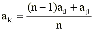
where: akl - an element of the new k-th "average" clashes, resulting from the merger of the i-th and j-th clashes;
n-1 is the number of clips already “merged” in the old i-th clutch;
ajl is an element of a new clink.
It is clear that, as soon as the program starts merging, the clips appear in the directory, the elements of which ail take on gradual values in the interval [-1, + 1]. (As in the factor analysis, the weight of the claw is determined by the formula Wj = Sa2iL) Empirically, by interpreting the results obtained with different thresholds P, we chose a threshold with an optimal value of p = 0.2 (for higher values of P in the catalog there are too many clicks According to our results, similar to each other and in terms of the content representing the variations of the main factor, which for 16PF turned out to be the anxiety factor (see [10], in press.).
It is clear that the introduction of “mergers” into the search program significantly modified the algorithm compared to its version, which was used earlier in the analysis of matrices of small sizes (for example, 17 × 17 [19]). The use of such a modification is inevitable with respect to the loose correlation matrices of high dimension (several hundreds of elements). With the help of mergers, it is possible to more accurately describe the main areas of clusters of points correlated with each other.
The volume of this message does not allow to dwell in detail on the interpretation of the clays we have identified when analyzing paragraphs 16PF. We only point out that their specificity as compared with the factors is that they almost always retain meaningful connections in the leading factors of weight. If, during factor analysis, the content of the main factors is extracted from the correlation matrix by subtracting the reproductive matrix (see the popular description of this operation in [16]), then with the key analysis, this elimination of the leading factors does not occur. The resulting catalog of clays is close to an oblique factorial solution, but, obviously, surpasses it in capacity, since it incorporates correlation information that goes beyond the orthogonal basis of the main factors.
According to the content, the selected clips have a certain conceptual novelty. Leading characteristics of individuality (secondary factors 16 PF - anxiety, exvia - invija, conformism, sensitivity, etc.) appear in their own finely nuanced variations, for example, the diagnostic construct “anxiety” is specified in the form of numerous variations associated with a variety of manifestations of anxiety in different subject areas and situations: these are “social anxiety” (in communication with people), “hypochondriac anxiety” (in relation to their somatic state), “anxiety of achievement” ( in relation to the risk of success or failure in activities), etc.
Studying the effectiveness of the klaikalysis algorithm developed by us, we carried out a special comparison of the results of cluster analysis and klike analysis applied to the same response array of 380 subjects for the 16PF test questionnaire (Form B). Revealed a significant coincidence of the largest clusters obtained by the method of the average distance, and the largest clays. (Coincidence was measured using the congruence factor (9), significance was estimated by chi-square). But the results of the klaik-analysis turned out to be more complete: among the clays, almost all clusters can be found, but not all clays are described as clusters. It is also important to note that the clays have a higher statistical stability with respect to the sample: when splitting the sample in half, the klaik-solution turned out to be more stable than the cluster-solution. Thus, relatively stable clutches can be obtained already on samples of small volume (from 100 to 200 subjects).
7. Block analysis
As J. Rask (1973) wittily observes, from a formal, mathematical point of view, there is no difference between the two inputs of the rectangular matrix “test points ×”. All analysis methods that are applicable to items are also applicable to the analysis of the relationship between subjects. In the latter case, pairwise correlations are calculated between the rows of the matrix | R |. For factor analysis, such an approach has long been known under the name of the P-variant (as opposed to the Q-variant - the analysis of issues).
Conveniently present | R | as a graph representing one set of vertices of Q - subjects - into another set of Q - questions (points). The unit in the cell of the matrix means the presence of an edge between the vertices of Pi and qj
We call a block in such a graph a pair of subsets P and Q such that for every Pi belonging to P, the image qj from Q has a prototype of the entire subset of P, that is, from each vertex P there is an edge to every vertex Q. If the corresponding rows P and columns Q in the matrix | R | grouped together, you get a rectangle (block) of cells containing only units (Table 2).
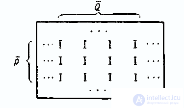
As is known from combinatorics (see [13]), in order to find the complete subgraph for some vertex Pi, the transposed vector-string <Ri> should be multiplied to the right of the matrix | R | according to the rules of matrix multiplication. In this case, it will mean a search for this subject pi such test subjects from which answered “right” to the same questions Q as the pi. Similarly, for the qi question, you can find all the Q questions that were answered “right” by the same subjects, but in this case, the transposed column vector <Qq> must be multiplied on the left by the matrix | R |.
These simple combinatorial considerations explain the basic idea of the block analysis algorithm that we developed. (Answers "incorrectly" are encoded in | R | with the values "-1".) This algorithm includes N iteration cycles (by the number N of the subjects or rows of the matrix | R |). In the course of the next i-cycle, the ith transposed (turned into a column) row of the matrix <R0i> = <Q0> is multiplied to the right of the matrix | R |. The resulting string <p '> is normalized (divided by the maximum of <p'>) and multiplied to the left by the matrix | R |. The new column vector <Q '> is multiplied to the right of | R |, and this continues until both <Qt + 1> and <Qt>, as well as <pt + 1> and <pt>, stabilize with negligible error. As a result, for each i-th subject, an approximate block is found, in which both subjects and items come in with different weights (similar to factor loads in factor analysis).
According to the program we wrote in the BASIC language, practical testing of the described algorithm was carried out on a mini-computer and the comparison of its results with the results of the usual algorithm for analyzing the main components. A significant coincidence was obtained: the most powerful blocks reproduced well the main components for the points. The advantage of the block algorithm is that it simultaneously gives factor weights for the subjects (the weight with which the subject entered the unit is evaluated), and also that it works much faster and more efficiently with respect to large matrices containing many small blocks ( multifactorial test questionnaires). The practical convenience of the block is that it simultaneously describes both the diagnostic construct (in the form of a set of items with weighting factors) and the subsample of subjects (of a certain gender, age, specialty) on which this construct was reproduced.
We believe that this type of algorithm belongs to the future in the analysis of centralized computer banks of psychodiagnostic information collected on some basic lists of questions in various areas of practical psychology.
Broad prospects are opening up for psychologists with the introduction of a centralized psychodiagnostic service in the future. In this case, the psychologist-practitioner writes out from the methodical center a so-called basic list of questions of a certain focus (for example, a characterological basic list, apparently, will include about 1000 questions). In his selective methodological study, the psychologist-practitioner collects the answers of his subjects to all the questions in the basic list and sends criterial information about the sample, as well as protocols with answers to the methodological center. The center, which has a powerful computational base, makes a computer analysis of the sent array, complements its data bank and sends the practical psychologist the analysis results, on the basis of which the practitioner selects a compact list of questions (30-100 points) for practical use for the purpose of mass express diagnostics.
Literature
Questions of psychology, No. 4, 1985. - P.126-134.

Comments
To leave a comment
Mathematical Methods in Psychology
Terms: Mathematical Methods in Psychology