Lecture
Optimization - modification of the system to improve its effectiveness. A system can be a single computer program, a digital device, a set of computers, or even an entire network, such as the Internet.
Programmers are constantly engaged in program optimization. This is the same integral part of the work as fixing bugs or refactoring. Usually, by saying "optimization", we mean the acceleration of the program. Despite the fact that optimization can also be understood as a reduction in the amount of RAM used or other resources (say, network traffic or battery charge), this article will focus on acceleration.
For a start, a little truths. Nobody is engaged in optimization until the customer comes (or a colleague from the QA department - it doesn’t matter) and says that the program is too slow in such a place. That is, first of all we write a program with simple and understandable code, test it properly and only then, if necessary , optimize it. It makes no sense to optimize the program if (1) everything works and everyone is satisfied, (2) after six months, the requirements for the program will change and the code will have to be rewritten.
Note: Perhaps, if you are writing a library, then you can take care of its optimization in advance.
Also, no one rushes to optimize the program until it becomes clear how fast it should work. The wording “the table should be rendered no longer than one second” is correct, and “the table should be drawn quickly” is not. That is, you should know in which case the work should be considered completed. You can not achieve a goal that is constantly changing. (But if the business does not want to understand this, well ... any whim for your money.)
Taking on the optimization, we find the very brake point and accelerate it. If the program is now running fast enough and nothing is broken, the goal is achieved. Otherwise, go to the first step. You can search for slow spots, for example, using the profiler, writing metrics to Graphite, debugging output with timestamps, or logging slow SQL queries. You can, of course, and at random, if at your disposal a lot of time.
We now turn directly to the methods. I suspect that some of them will surprise you, nevertheless ...
Software update . This may seem incredible, but switching to the latest version of any library, DBMS, Erlang virtual machine or Linux kernel used in a project can significantly increase the speed of your application. Simple and usually quick fix.
Setting the environment . The used DBMS or operating system may not be configured correctly. The default settings for MySQL and PostgreSQL suggest that you are trying to run the DBMS on the initial file. One of my colleagues told me how once in his practice, the application was significantly accelerated by simply trying various JVM options. This method is even simpler than software update. However, it is necessary to use it, for obvious reasons, after the update. Or in case the update is impossible for some reason in the foreseeable future.
Removing unnecessary functionality . You can increase the speed of your application by throwing out unnecessary code. Sometimes it turns out that the program does something unnecessary or not very necessary. Perhaps one of the problems solved has lost its relevance. Sometimes the customer, instead of the real problem, describes the programmer his vision of solving it, and the programmer, because of his inexperience, simply codes this solution. In the meantime, solving this problem can be much easier. Sometimes a functional overgrows crutches and props. In this case, it makes sense to implement the functionality from scratch, and throw out the old solution.
Buying a new iron . What is not a method? It is often much faster and cheaper to buy new hardware than to optimize the program code. In some cases, doubling the number of processor cores can double the speed of the program. You can purchase additional RAM and store data in it, instead of taking it from disk or transferring it over the network. You can transfer the database to SSD. If the program is scaled horizontally, you can purchase a dozen servers.
Memoisation and caching . We now turn to “real” optimizations. Memoization is the preservation of the value returned by a function for given arguments. Caching is the preservation of the results of anything. For example, web pages or monthly reports can be cached. Caching may not be applicable if the cached data is updated quickly. Also in the context of caching, the problem of cache invalidation often arises. In the context of memoization, such a problem does not arise, since memoizations usually undergo pure functions , that is, functions without side effects, the return value of which depends only on the arguments. Memoisation and caching are efficient and easy to implement, but improper caching can prevent program scaling. When adding to your application cache, think about how you will manage it when the program runs in two or more instances.
Parallelization . Parallelization can be a simple or complex operation, depending on. For example, in Erlang, many tasks can be easily parallelized by writing literally a dozen lines of code. And in Scala, you can easily use parallel collections instead of regular ones. However, some tasks cannot be solved in parallel in nature. And if the program runs on a single-core processor, paralleling does nothing. Nondeterministic functions and functions with side effects complicate the use of this optimization, which is another reason for writing pure functions. When writing the web or some backends, parallelization is not always possible, since it is impossible to take all the kernels into processing a single user request, thereby blocking the processing of other requests.
Load distribution If the load on the DBMS is low, you can use triggers or snapshots, thereby relieving the application itself and reducing traffic. Or, on the contrary, you can transfer all the logic to the application by unloading the DBMS. To build reports, create backup copies and perform other heavy operations on the DBMS, it makes sense to have a special replica. DBMS can be configured so that different tables are stored on different physical disks. You can give the user a static page with JavaScript and communicate with him exclusively using the REST API. Let him generate HTML for himself. Static content can be kept on a separate domain. This will reduce the traffic, since no cookies will be sent to this domain. There is no need to gzip / encrypt data in Apache or even in the application itself, if nginx can cope with this task much better. Using sharding, you can distribute the load across multiple database replicas, Erlang processes, or Memcached instances.
Lazy computing . Roughly speaking, lazy calculations are when an anonymous function is returned instead of a specific value, which, when called, calculates this value. In a number of programming languages, lazy calculations are supported at the syntax level. The trick is to calculate the value immediately before using it. Imagine the situation when we give the data in CSV format and the user can specify a filter that determines which columns should be transferred. In this case, lazy calculations are very helpful. If it turns out that the value is not really needed, we will save time spent on its calculation. However, it should be noted that lazy calculations lead to an increase in the amount of memory used and can work poorly with dirty functions.
Deferred settlement . Why consider something right now, if it can be done later? When processing an HTTP request, we can instantly return OK to the user, and perform the actual work in the background process. If the request is very important, we can put it in the persistent task queue processed by cron. Or a group of continuously working processes. In the latter case, we even have good chances to get a horizontal scaling and, accordingly, a real increase in speed, and not only visible. In addition, deferred tasks may be similar. For example, they need the same data from the database. In this case, with deferred processing of N tasks in one bundle, you can go to the database N times less.
More suitable algorithms and data structures. Quicksort is faster than bubble sort, and elliptic curves are faster than RSA. If you want to verify that an element belongs to a set, you should use hash tables, rather than single-linked lists. Correct indexes and denormalization of the database schema can significantly reduce the execution time of SQL queries. If you need to synchronize some data, instead of sending it completely with each change, it is better to use the snapshot + updates scheme.
Approximation . This is almost a case of a more suitable algorithm, but with a loss of accuracy. Instead of long arithmetic, you can often get by with ordinary floats. When collecting statistics, data can be sent via UDP instead of TCP. Let a small part of the packages not reach, and part - come twice. When collecting statistics, changing numbers is more important than specific values. Also, for example, there is no need to build a graph for all points, if you can take a subset of them and build a Bezier curve. Instead of a costly calculation of the median, you can often calculate the average.
Rewriting to another language . It may well be that the program is significantly hampered by garbage collection or, say, type checking at runtime. Rewriting small parts of a program from Ruby to Scala or from Erlang to OCaml can speed up this program. If the rewritable piece of code is simple enough, you can rewrite it in C or C ++ with a slight risk. This method should be used very carefully. It leads to the emergence of a zoo programming languages, which complicates support for the project. The method may not work, for example, because of the overhead of converting data from one view to another. It can also be dangerous. For example, an error in the NIF can lead to the fall of the entire Erlang virtual machine, and not a single process.
In conclusion, I want to note that the above classification is very, very conditional. Obviously, the line between parallelization and load distribution or deferred calculations and lazy calculations is very blurred.
Some tasks can often be performed more efficiently. For example, a C program that sums up all integers from 1 to N:
 int i, sum = 0;
 for (i = 1; i <= N; i ++)
   sum + = i;
Assuming that there is no overflow, this code can be rewritten as follows using the appropriate mathematical formula:
int sum = (N * (N + 1)) / 2;
The concept of "optimization" usually implies that the system retains the same functionality. However, significant performance improvements can often be achieved by removing redundant functionality. For example, if we assume that the program does not need to support more than 100 items when entering, then it is possible to use static memory allocation instead of a slower dynamic one.
Optimization mainly focuses on single or repeated runtime, memory usage, disk space, bandwidth, or some other resource. This usually requires a compromise - one parameter is optimized at the expense of others. For example, increasing the size of a software cache improves performance of the runtime, but also increases memory consumption. Other common tradeoffs include code transparency and expressiveness, almost always at the cost of de-optimization. Complex specialized algorithms require more effort to debug and increase the likelihood of errors.
In operations research, optimization is the problem of determining the input values of a function for which it has a maximum or minimum value. Sometimes restrictions are imposed on these values, such a task is known as limited optimization .
In programming, optimization usually means modifying the code and its compilation settings for a given architecture to produce more efficient software.
Typical problems have such a large number of possibilities that programmers usually can only use a “reasonably good” solution.
Optimization requires finding a bottleneck (eng. Bottleneck - bottleneck): a critical part of the code that is the main consumer of the required resource. Improving about 20% of the code sometimes entails a change in 80% of the results (see also the Pareto principle). To search for bottlenecks special programs are used - profilers. Leakage of resources (memory, descriptors, etc.) can also lead to a drop in the speed of program execution, special programs are also used to find them (for example, BoundsChecker).
The architectural design of the system especially affects its performance. The choice of algorithm affects the efficiency more than any other design element. More complex algorithms and data structures can operate well with a large number of elements, while simple algorithms are suitable for small amounts of data — the overhead of initializing a more complex algorithm may outweigh the benefits of using it.
The more memory a program uses, the faster it is usually executed. For example, a filter program typically reads each line, filters and displays this line directly. Therefore, it uses memory only to store a single line, but its performance is usually very poor. Performance can be significantly improved by reading the entire file and writing the filtered result afterwards, but this method uses more memory. Result caching is also efficient, but requires more memory to use.
Optimization of the cost of processor time is especially important for computational programs in which mathematical calculations have a large proportion. Here are some optimization techniques that a programmer can use when writing source code for a program.
In many programs, some of the data objects must be initialized , that is, they must be assigned initial values. Such an assignment is performed either at the very beginning of the program, or, for example, at the end of a cycle. Proper object initialization saves valuable CPU time. So, for example, when it comes to initializing arrays, using a loop is likely to be less effective than declaring this array as a direct assignment.
In the case when a significant part of the program's working time is devoted to arithmetic calculations, considerable reserves for increasing the program speed are hidden in the correct programming of arithmetic (and logical) expressions. It is important that various arithmetic operations vary considerably in speed. In most architectures, the fastest addition and subtraction operations are. Multiplication is slower, then division goes. For example, calculating the value of an expression  where
where  - constant, for floating-point arguments, is faster in the form
  where
where  - constant, calculated at the compilation of the program (in fact, the slow division operation is replaced by the fast multiplication operation). For integer argument
  expression evaluation
  faster to produce in the form
  (the multiplication operation is replaced by the addition operation) or using the left shift operation (which ensures that not all processors win). Such optimizations are called lowering the strength of operations. Multiplying integer arguments by a constant on x86 processors can be efficiently performed using assembler commands LEA, SHL and ADD instead of using the MUL / IMUL commands:
 ;  Source operand in the EAX register
 ADD EAX, EAX;  multiplication by 2

 LEA EAX, [EAX + 2 * EAX];  multiplication by 3

 SHL EAX, 2;  multiplication by 4

 LEA EAX, [4 * EAX];  another embodiment of multiplying by 4

 LEA EAX, [EAX + 4 * EAX];  multiplication by 5

 LEA EAX, [EAX + 2 * EAX];  multiplication by 6
 ADD EAX, EAX

 ;  etc.
Such optimizations are micro-architectural and are usually produced by the optimizing compiler transparently to the programmer.
Relatively long time is spent on accessing subroutines (passing parameters via the stack, saving registers and return addresses, calling copy constructors). If the subroutine contains a small number of operations, it can be realized substitutes (Engl. Inline ) — все её операторы копируются в каждое новое место вызова (существует ряд ограничений на inline-подстановки: например, подпрограмма не должна быть рекурсивной). Это ликвидирует накладные расходы на обращение к подпрограмме, однако ведет к увеличению размера исполняемого файла. Само по себе увеличение размера исполняемого файла не является существенным, однако в некоторых случаях исполняемый код может выйти за пределы кэша команд, что повлечет значительное падение скорости исполнения программы. Поэтому современные оптимизирующие компиляторы обычно имеют настройки оптимизации по размеру кода и по скорости выполнения.
Быстродействие также зависит и от типа операндов. Например, в языке Turbo Pascal, ввиду особенностей реализации целочисленной арифметики, операция сложения оказывается наиболее медленной для операндов типа Byte и ShortInt: несмотря на то, что переменные занимают один байт, арифметические операции для них двухбайтовые и при выполнении операций над этими типами производится обнуление старшего байта регистров и операнд копируется из памяти в младший байт регистра. Это и приводит к дополнительным затратам времени.
Программируя арифметические выражения, следует выбирать такую форму их записи, чтобы количество «медленных» операций было сведено к минимуму. Рассмотрим такой пример. Пусть необходимо вычислить многочлен 4-й степени:

При условии, что вычисление степени производится перемножением основания определенное число раз, нетрудно найти, что в этом выражении содержится 10 умножений («медленных» операций) и 4 сложения («быстрых» операций). Это же самое выражение можно записать в виде:

Такая форма записи называется схемой Горнера. В этом выражении 4 умножения и 4 сложения. Общее количество операций сократилось почти в два раза, соответственно уменьшится и время вычисления многочлена. Подобные оптимизации являются алгоритмическими и обычно не выполняются компилятором автоматически.
Различается и время выполнения циклов разного типа. Время выполнения цикла со счетчиком и цикла с постусловием при всех прочих равных условиях , цикл с предусловием выполняется несколько дольше (примерно на 20-30 %).
When using nested loops, it should be borne in mind that the CPU time spent on processing such a construction may depend on the order of the nested loops. For example, a nested loop with a counter in the Turbo Pascal language:
   for j: = 1 to 100000 do
      for k: = 1 to 1000 do a: = 1;
|
   for j: = 1 to 1000 do
      for k: = 1 to 100000 do a: = 1;
|
The cycle in the left column is about 10% longer than the right.
At first glance, both in the first and in the second case, the assignment statement is executed 100,000,000 times and the time spent on it should be the same in both cases. But it is not. Объясняется это тем, что инициализации цикла (обработка процессором его заголовка с целью определения начального и конечного значений счётчика, а также шага приращения счётчика) требует времени. В первом случае 1 раз инициализируется внешний цикл и 100 000 раз — внутренний, то есть всего выполняется 100 001 инициализация. Во втором случае таких инициализаций оказывается всего лишь 1001.
Аналогично ведут себя вложенные циклы с предусловием и с постусловием. Можно сделать вывод, что при программировании вложенных циклов по возможности следует делать цикл с наибольшим числом повторений самым внешним, а цикл с наименьшим числом повторений — самым внутренним.
Если в циклах содержатся обращения к памяти (обычно при обработке массивов), для максимально эффективного использования кэша и механизма аппаратной предвыборки данных из памяти (англ. Hardware Prefetch ) порядок обхода адресов памяти должен быть по возможности последовательным. Классическим примером подобной оптимизации является смена порядка следования вложенных циклов при выполнении умножения матриц.
При вычислении сумм часто используются циклы, содержащие одинаковые операции, относящиеся к каждому слагаемому. Это может быть, например, общий множитель (язык Turbo Pascal):
  sum := 0;
  for i := 1 to 1000 do
    sum := sum + a * x[i];
|
  sum := 0;
  for i := 1 to 1000 do
    sum := sum + x[i];
  sum := a * sum;
|
Вторая форма записи цикла оказывается более экономной.
Оптимизация инвариантных фрагментов кода тесно связана с проблемой оптимального программирования циклов. Внутри цикла могут встречаться выражения, фрагменты которых никак не зависят от управляющей переменной цикла. Их называют инвариантными фрагментами кода. Современные компиляторы часто определяют наличие таких фрагментов и выполняют их автоматическую оптимизацию. Такое возможно не всегда, и иногда производительность программы зависит целиком от того, как запрограммирован цикл. В качестве примера рассмотрим следующий фрагмент программы (язык Turbo Pascal):
   for i := 1 to n do
   begin
    ...
       for k := 1 to p do
             for m := 1 to q do
             begin
                   a[k, m] := Sqrt(x * k * m - i) + Abs(u * i - x * m + k);
                   b[k, m] := Sin(x * k * i) + Abs(u * i * m + k);
             end;
    ...
   am := 0;
   bm := 0;
   for k := 1 to p do
             for m := 1 to q do
             begin
                   am := am + a[k, m] / c[k];
                   bm := bm + b[k, m] / c[k];
             end;
   end;
Здесь инвариантными фрагментами кода являются слагаемое Sin(x * k * i) в первом цикле по переменной m и операция деления на элемент массива c[k] во втором цикле по m. Значения синуса и элемента массива не изменяются в цикле по переменной m, следовательно, в первом случае можно вычислить значение синуса и присвоить его вспомогательной переменной, которая будет использоваться в выражении, находящемся внутри цикла. Во втором случае можно выполнить деление после завершения цикла по m. Таким образом, можно существенно сократить количество трудоёмких арифметических операций.
Большинство программистов представляют вычислительную систему как процессор, который выполняет инструкции, и память, которая хранит инструкции и данные для процессора. В этой простой модели память представляется линейным массивом байтов и процессор может обратиться к любому месту в памяти за константное время. Хотя это эффективная модель для большинства ситуаций, она не отражает того, как в действительности работают современные системы.
В действительности система памяти образует иерархию устройств хранения с разными ёмкостями, стоимостью и временем доступа. Регистры процессора хранят наиболее часто используемые данные. Маленькие быстрые кэш-памяти, расположенные близко к процессору, служат буферными зонами, которые хранят маленькую часть данных, расположеных в относительно медленной оперативной памяти. Оперативная память служит буфером для медленных локальных дисков. А локальные диски служат буфером для данных с удалённых машин, связанных сетью.
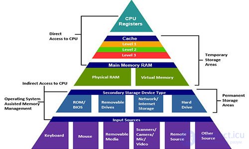
Иерархия памяти работает, потому что хорошо написанные программы имеют тенденцию обращаться к хранилищу на каком-то конкретном уровне более часто, чем к хранилищу на более низком уровне. Так что хранилище на более низком уровне может быть медленнее, больше и дешевле. В итоге мы получаем большой объём памяти, который имеет стоимость хранилища в самом низу иерархии, но доставляет данные программе со скоростью быстрого хранилища в самом верху иерархии.
Как программист, вы должны понимать иерархию памяти, потому что она сильно влияет на производительность ваших программ. Если вы понимаете как система перемещает данные вверх и вниз по иерархии, вы можете писать такие программы, которые размещают свои данные выше в иерархии, так что процессор может получить к ним доступ быстрее.
В этой статье мы исследуем как устройства хранения организованы в иерархию. Мы особенно сконцентрируемся на кэш-памяти, которая служит буферной зоной между процессором и оперативно памятью. Она оказывает наибольшее влияние на производительность программ. Мы введём важное понятие локальности , научимся анализировать программы на локальность, а также изучим техники, которые помогут увеличить локальность ваших программ.
На написание этой статьи меня вдохновила шестая глава из книги Computer Systems: A Programmer's Perspective . В другой статье из этой серии, «Оптимизация кода: процессор», мы также боремся за такты процессора.
Consider two functions that summarize the elements of a matrix. They are almost the same, only the first function bypasses the elements of the matrix line by line, and the second - in columns.
int matrixsum1 (int size, int M [] [size]) {int sum = 0; for (int i = 0; i // go around line by line }} return sum; } int matrixsum2 (int size, int M [] [size]) {int sum = 0; for (int i = 0; i // go around the columns }} return sum; }
Both functions perform the same number of processor instructions. But on a machine with a Core i7 Haswell, the first function runs 25 times faster for large matrices. This example well demonstrates that memory matters too . If you evaluate the effectiveness of programs only in terms of the number of instructions to be executed, you can write very slow programs.
Data has an important property that we call locality . When we work on the data, it is desirable that they are in the memory next. Traversing the matrix in columns has poor locality, because the matrix is stored in memory line by line. We'll talk about locality below.
The modern memory system forms a hierarchy from fast types of memory of small size to slow types of memory of large size. We say that a particular hierarchy level caches or is a cache for data located at a lower level. This means that it contains copies of data from a lower level. When the processor wants to get some data, it first searches for it at the fastest high levels. And descends to lower, if not can find.
At the top of the hierarchy are the registers of the processor. Access to them takes 0 cycles, but there are only a few of them. Next comes a few kilobytes of first-level cache, access to which takes about 4 clock cycles. Then comes a couple of hundred kilobytes of a slower second-level cache. Then a few megabytes of third-level cache. It is much slower, but still faster than RAM. Next is a relatively slow RAM.
RAM can be considered as a cache for a local disk. Disks are workhorses among storage devices. They are big, slow and cheap. The computer loads files from disk into RAM when it is going to work on them. The gap in access time between the RAM and the disk is enormous. The disk is tens of thousands of times slower than RAM, and millions of times slower than the first level cache. It is more profitable to turn several thousand times to RAM than once to a disk. This knowledge is supported by such data structures as B-trees , which try to place more information in the RAM, trying to avoid accessing the disk at any cost.
The local disk itself can be considered as a cache for data located on remote servers. When you visit a website, your browser saves images from a web page to disk so that you do not need to download them when you visit them again. There are lower memory hierarchies. Large data centers, such as Google, store large amounts of data on tape media that is stored somewhere in warehouses, and when needed, must be attached manually or by a robot.
The modern system has approximately the following characteristics:
| Cache type | Access time (cycles) | Cache size |
|---|---|---|
| Registers | 0 | dozens of pieces |
| L1 cache | four | 32 KB |
| L2 cache | ten | 256 KB |
| L3 cache | 50 | 8 MB |
| RAM | 200 | 8 GB |
| Disk buffer | 100'000 | 64 MB |
| Local disk | 10'000'000 | 1000 GB |
| Remote servers | 1'000'000'000 | ∞ |
Fast memory is very expensive, and slow memory is very cheap. It is a great idea for system architects to combine large sizes of slow and cheap memory with small sizes that are fast and expensive. Thus, the system can operate at a fast memory speed and have a slow cost. Let's see how it works out.
Suppose your computer has 8 GB of RAM and a 1000 GB disk. But think that you do not work with all the data on the disk at one time. You load the operating system, open a web browser, text editor, a couple of other applications, and work with them for several hours. All these applications are placed in RAM, so your system does not need to access the disk. Then, of course, you close one application and open another, which you have to load from disk into RAM. But it takes a couple of seconds, after which you work with this application for several hours without accessing the disk. You do not really notice a slow disk, because at one moment you are working only with a small amount of data that is cached in RAM. It makes no sense for you to spend huge amounts of money on installing 1024 GB of RAM into which you could load the contents of the entire disk. If you had done this, you would have hardly noticed any difference in the work, it would be “money down the drain.”
The same is true for small processor caches. Suppose you need to perform calculations on an array that contains 1000 elements of type int . Such an array occupies 4 KB and is completely placed in the cache of the first level with a size of 32 KB. The system understands that you started working with a certain piece of RAM. It copies this piece into the cache, and the processor quickly performs actions on this array, enjoying the speed of the cache. Then the modified array from the cache is copied back into RAM. Increasing the speed of RAM to the speed of the cache would not give a tangible increase in performance, but would increase the cost of the system hundreds and thousands of times. But all this is true only if the programs have good locality.
Locality is the main concept of this article. As a rule, programs with good locality run faster than programs with poor locality. Locality is of two types. When we refer to the same place in memory many times, this is a temporary locality . When we access data, and then we access other data that are located in memory next to the original data, this is spatial locality .
Consider a program that summarizes the elements of an array:
 int sum (int size, int A [])
 {
     int i, sum = 0;

     for (i = 0; i
In this program, the call to the variables sum and i occurs at each iteration of the loop. They have a good temporary locality and will be located in fast processor registers. Elements of array A have a bad temporal locality, because we refer to each element only once. But then they have good spatial locality - by touching one element, we then touch the elements next to it. All the data in this program have either good temporal locality or good spatial locality, so we say that the program generally has good locality. When the processor reads data from memory, it copies it to its cache, while deleting other data from the cache. What kind of data he chooses to delete the topic is difficult. But the result is that if some data is accessed frequently, they are more likely to remain in the cache. This is a benefit from temporal locality. It is better for the program to work with fewer variables and to access them more often. Data movement between levels of hierarchy is performed by blocks of a certain size. For example, the Core i7 Haswell processor moves data between its caches in blocks of 64 bytes. Consider a specific example. We run the program on a machine with the aforementioned processor. We have an array v containing 8-byte elements of type long . And we sequentially go around the elements of this array in a loop. When we read v [0] , it is not in the cache, the processor reads it from RAM to the cache with a block of 64 bytes in size. That is, elements v [0] - v [7] are sent to the cache. Next we go around the elements v [1] , v [2] , ..., v [7] . All of them will be in the cache and we will get access to them quickly. Then we read the element v [8] , which is not in the cache. The processor copies the elements v [8] - v [15] into the cache. We quickly go around these elements, but do not find the element v in the cache [16] . And so on. Therefore, if you read some bytes from memory, and then read the bytes next to them, they will most likely be in the cache. This is a benefit of spatial locality. It is necessary to strive at each stage of calculation to work with the data that are located in the memory nearby. It is advisable to bypass the array sequentially by reading its elements one by one. If you need to bypass the elements of the matrix, it is better to bypass the matrix line by line, rather than in columns. This gives a good spatial locality. Now you can understand why the matrixsum2 function was slower than the matrixsum1 function. A two-dimensional array is located in memory line by line: first the first line is located, immediately after it comes the second one and so on. The first function read the elements of the matrix line by line and moved sequentially from memory, as if bypassing one large one-dimensional array. This function basically read the data from the cache. The second function went from line to line, reading one element at a time. She seemed to leap from memory from left to right, then return to the beginning and again began to jump from left to right. At the end of each iteration, she clogged the cache with the last lines, so she did not find the first lines at the beginning of the next iteration. This function basically read data from RAM.
As programmers, you should try to write code that is cache-friendly . As a rule, the main volume of calculations is performed only in a few places of the program. Usually these are several key functions and loops. If there are nested loops, then attention should be focused on the innermost of the loops, because the code is executed there most often. These places of the program also need to be optimized, trying to improve their locality. Matrix calculations are very important in signal analysis and scientific computing applications. If programmers have the task to write the matrix multiplication function, then 99.9% of them will write it like this:
 void matrixmult1 (int size, double A [] [size], double B [] [size], double C [] [size])
 {
     double sum;

     for (int i = 0; i
This code literally repeats the mathematical definition of matrix multiplication. We go around all the elements of the final matrix line by line, calculating each of them one by one. There is one inefficiency in the code, this is the expression B [k] [j] in the innermost loop. We go around matrix B by columns. It would seem that nothing can be done about it and will have to accept. But there is a way out. You can rewrite the same calculation differently:
 void matrixmult2 (int size, double A [] [size], double B [] [size], double C [] [size])
 {
     double r;

     for (int i = 0; i
Now the function looks very strange. But she does absolutely the same thing. Only we do not calculate each element of the final matrix at a time; we sort of calculate the elements partly at each iteration. But the key feature of this code is that in the internal loop we go around both matrices line by line. On the machine with the Core i7 Haswell, the second function works 12 times faster for large matrices. You need to be a really wise programmer to organize the code in this way.
There is a technique called blocking . Suppose you need to perform a calculation on a large amount of data that does not all fit in the high-level cache. You break this data into smaller blocks, each of which is cached. Perform calculations on these blocks separately and then merge the result. You can demonstrate this by example. Suppose you have a directed graph presented in the form of an adjacency matrix. This is such a square matrix of zeros and ones, so that if the element of the matrix with the index (i, j) is equal to one, then there is a face from the vertex of the graph i to the vertex j . You want to turn this directed graph into undirected. That is, if there is a face (i, j) , then the opposite face (j, i) should appear. Note that if the matrix is represented visually, then the elements (i, j) and (j, i) are symmetric with respect to the diagonal. This transformation is easy to implement in the code:
 convert1 void (int size, int G [] [size])
 {
     for (int i = 0; i
Blocking appears naturally. Imagine a large square matrix in front of you. Now excise this matrix with horizontal and vertical lines to break it up, say, into 16 equal blocks (four rows and four columns). Choose any two symmetric blocks. Please note that all elements in one block have their own symmetrical elements in another block. This suggests that the same operation can be performed on these blocks in turn. In this case, at each stage we will work only with two blocks. If the blocks are made small enough, they will fit in the high level cache. Express this idea in code:
convert2 void (int size, int G [] [size])
{
int block_size = size / 12; // split into 12 * 12 blocks
// imagine what is divided without remainder
for (int ii = 0; ii // index i for a block takes values [ii, ii + block_size)
int i_end = ii + block_size;
int j_start = jj; // index j for a block takes values [jj, jj + block_size)
int j_end = jj + block_size;
// go around the block
for (int i = i_start; i
It should be noted that blocking does not improve performance on systems with powerful processors that do a good prefetch. On systems that do not prefetch, blocking can greatly increase performance. On a machine with a Core i7 Haswell processor, the second function does not run faster. On a machine with a simpler Pentium 2117U processor, the second function is performed 2 times faster. On machines that do not prefetch, performance would improve even more.
Everyone knows from the courses on algorithms that you need to choose good algorithms with the least complexity and avoid bad algorithms with high complexity. But these difficulties evaluate the implementation of the algorithm on a theoretical machine created by our thought. On real machines, a theoretically bad algorithm can run faster than a theoretically good one. Remember that getting data from RAM takes 200 ticks, and 4 ticks from the first level cache is 50 times faster. If a good algorithm often touches memory, and a bad algorithm places its data in the cache, a good algorithm can run slower than a bad one. Also, a good algorithm can run worse on a processor than a bad one. For example, a good algorithm introduces data dependency and cannot load a processor pipeline. A bad algorithm is deprived of this problem and sends a new instruction to the pipeline on every clock cycle. In other words, the complexity of the algorithm is not all. How the algorithm will run on a specific machine with specific data matters. Imagine that you need to implement a queue of integers, and new elements can be added to any position in the queue. You choose between two implementations: an array and a linked list. To add an element to the middle of the array, you need to move half the array to the right, which takes linear time. To add an element to the middle of the list, you need to go through the list to the middle, which also takes linear time. You think that since they have the same complexity, it is better to choose a list. Moreover, the list has one good property. The list can grow without limit, and the array will have to expand when it is full. For example, we implemented a queue with a length of 1000 elements in both ways. And we need to insert an item in the middle of the queue. The elements of the list are randomly scattered in memory, so to get around 500 elements, we need 500 * 200 = 100'000 cycles. The array is located in memory sequentially, which allows us to enjoy the first-level cache speed. Using several optimizations, we can move the elements of the array, spending 1-4 clocks per element. We will move half of the array to a maximum of 500 * 4 = 2000 cycles. That is 50 times faster. If in the previous example all the additions were to the top of the queue, the implementation with the linked list would be more efficient. If a fraction of the additions would be somewhere in the middle of the queue, implementing as an array could be the best choice. We would spend tacts on some operations and save tacts on others. And in the end, could remain the winner.
The memory system is organized as a hierarchy of storage devices with small and fast devices at the top of the hierarchy and large and slow devices at the bottom. Programs with good locality work with data from processor caches. Programs with poor locality work with data from relatively slow RAM. Programmers who understand the nature of the memory hierarchy can structure their programs so that the data is located as high as possible in the hierarchy and the processor receives them faster. In particular, the following techniques are recommended:

NB: logarithmic scale!
Преждевременная пессимизация Легко на себя, легко по коду: при прочих равных условиях, особенно в отношении сложности кода и удобочитаемости, некоторые эффективные шаблоны проектирования и идиомы кодирования должны просто естественным образом вытекать из ваших кончиков пальцев и писать их сложнее, чем пессимизированные альтернативы. Это не преждевременная оптимизация; он избегает безнадежной пессимизации. - Херб Саттер, Андрей Александреску. Всякий раз, когда нам нужно оптимизировать код, мы должны профилировать его, просто и просто. Тем не менее, иногда имеет смысл просто знать номера шаров для относительных затрат на некоторые популярные операции, поэтому вы не будете делать крайне неэффективные вещи с самого начала (и, надеюсь, позже не понадобится профилировать программу ).
Итак, здесь идет речь - инфографика, которая должна помочь оценить затраты на определенные операции в цикле тактовых импульсов ЦП и отвечать на такие вопросы, как «эй, сколько обычно читается L2?». Хотя ответы на все эти вопросы более или менее известны, я не знаю ни одного места, где все они перечислены и представлены в перспективе. Также отметим, что, хотя перечисленные номера, строго говоря, применяются только к современным процессорам x86 / x64, ожидается, что аналогичные модели относительных эксплуатационных затрат будут наблюдаться на других современных процессорах с большими многоуровневыми кэшами (такими как ARM Cortex A или SPARC); с другой стороны, MCU (включая ARM Cortex M) различны, поэтому некоторые из шаблонов могут быть разными.
И последнее, но не менее важное: слово осторожности: все оценки здесь являются лишь показаниями на порядок; однако, учитывая масштаб различий между различными операциями, эти показания могут по-прежнему использоваться (по крайней мере, следует иметь в виду избегать «преждевременной пессимизации»).
С другой стороны, я все еще уверен, что такая диаграмма полезна, чтобы не говорить о том, что «эй, вызовы виртуальных функций ничего не стоят» - что может быть или не быть истинным в зависимости от того, как часто вы их называете. Вместо этого, используя инфографику выше, вы сможете увидеть, что
если вы вызываете свою виртуальную функцию 100K раз в секунду на процессоре 3GHz - это, вероятно, не будет стоить вам более 0,2% от общего объема вашего процессора; однако, если вы вызываете одну и ту же виртуальную функцию 10M раз в секунду, это легко означает, что виртуализация поглощает двузначные проценты вашего ядра процессора.
Другой способ приблизиться к одному и тому же вопросу - сказать, что «эй, я вызываю виртуальную функцию один раз за кусок кода, который составляет 10000 циклов, поэтому виртуализация не будет потреблять более 1% от времени программы», - но вы все равно нужен какой-то способ увидеть порядок величины связанных затрат - и приведенная выше диаграмма по-прежнему будет полезна .
latency numbers every programmer should know 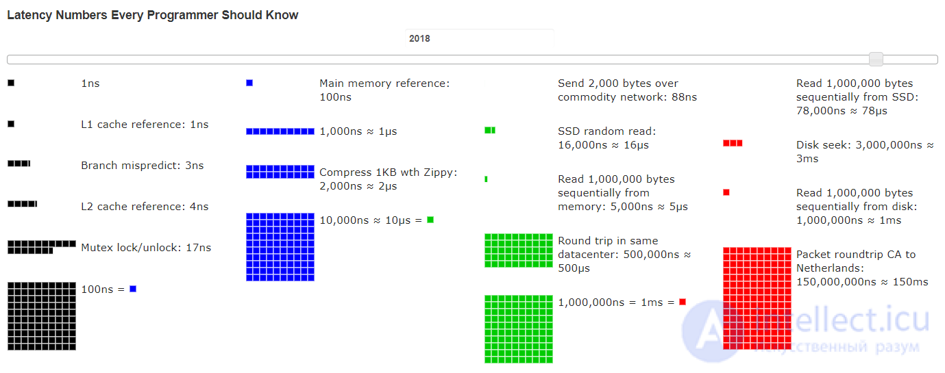
L1 cache reference ......................... 0.5 ns
Branch mispredict ............................ 5 ns
L2 cache reference ........................... 7 ns
Mutex lock/unlock ........................... 25 ns
Main memory reference ...................... 100 ns
Compress 1K bytes with Zippy ............. 3,000 ns = 3 µs
Send 2K bytes over 1 Gbps network ....... 20,000 ns = 20 µs
SSD random read ........................ 150,000 ns = 150 µs
Read 1 MB sequentially from
продолжение следует...
Часть 1 Methods of optimization programs. Latency numbers every programmer should know
Часть 2 - Methods of optimization programs. Latency numbers every programmer should

Comments
To leave a comment
Highly loaded projects. Theory of parallel computing. Supercomputers. Distributed systems
Terms: Highly loaded projects. Theory of parallel computing. Supercomputers. Distributed systems