Lecture
Machine Turinga (MT) - abstract artist (abstract computer). It was proposed by Alan Turing in 1936 to formalize the concept of an algorithm.
The Turing machine is an extension of the finite state machine and, according to the Church-Turing thesis, is able to imitate all the performers (using the transition rules), in any way implementing the step-by-step calculation process, in which each step of the calculation is quite elementary.
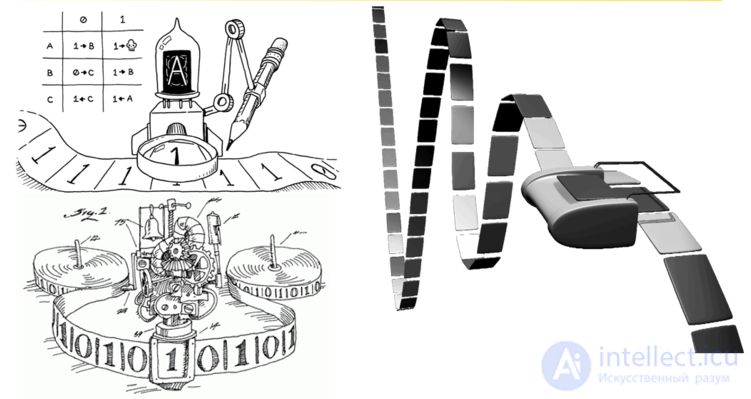
Artistic representation of the Turing machine
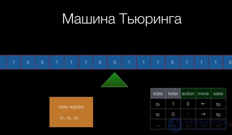
The Turing machine includes an unrestricted tape in both directions (Turing machines are possible that have several endless tapes), divided into cells, and a control device (also called a write-read head ( GZCH )) that can be in one of a variety of states . The number of possible states of the control device is of course and precisely specified.
The control device can move left and right along the tape, read and write the symbols of some finite alphabet in cells. A special empty symbol is selected that fills all cells of the tape, except for those of them (of finite number) on which the input data is written.
The control device operates according to the transition rules , which represent the algorithm implemented by this Turing machine. Each transfer rule instructs the machine, depending on the current state and the symbol observed in the current cell, to write a new symbol into this cell, switch to a new state and move one cell to the left or right. Some states of the Turing machine can be marked as terminal , and the transition to any of them means the end of the work, the stopping of the algorithm.
A Turing machine is called deterministic if each combination of a state and a ribbon symbol in the table corresponds to no more than one rule. If there is a “ribbon symbol - state” pair, for which there are 2 or more commands, such a Turing machine is called non-deterministic .
A specific Turing machine is specified by enumerating the elements of the set of letters of the alphabet A, the set of states Q, and the set of rules by which the machine operates. They have the form: q i a j → q i1 a j1 d k (if the head is in the state q i , and the letter a j is written in the monitored cell, then the head changes to the state q i1 , a j1 is written in the cell instead of a j the head makes the movement d k , which has three options: on the cell to the left (L), on the cell to the right (R), to stay in place (N)). For each possible configuration i , a j > there is exactly one rule (for a non-deterministic Turing machine there may be more rules). There are no rules only for the final state, once in which the car stops. In addition, it is necessary to specify the final and initial states, the initial configuration on the tape and the location of the machine head.
Let us give an example of MT for multiplying numbers in a unary number system. The rule “q i a j → q i1 a j1 R / L / N” should be understood as follows: q i is the state in which this rule is executed, a j is the data in the cell in which the head is located, q i1 is the state in which you need to go, a j1 - what you need to write to the cell, R / L / N - the command to move.
The machine works according to the following set of rules:
| q 0 | q 1 | q 2 | q 3 | q 4 | q 5 | q 6 | q 7 | q 8 | |
|---|---|---|---|---|---|---|---|---|---|
| one | q 0 1 → q 0 1R | q 1 1 → q 2 aR | q 2 1 → q 2 1L | q 3 1 → q 4 aR | q 4 1 → q 4 1R | q 7 1 → q 2 aR | |||
| × | q 0 × → q 1 × R | q 2 × → q 3 × L | q 4 × → q 4 × R | q 6 × → q 7 × R | q 8 × → q 9 × N | ||||
| = | q 2 = → q 2 = L | q 4 = → q 4 = R | q 7 = → q 8 = L | ||||||
| a | q 2 a → q 2 aL | q 3 a → q 3 aL | q 4 a → q 4 aR | q 6 a → q 6 1R | q 7 a → q 7 aR | q 8 a → q 8 1L | |||
| * | q 0 * → q 0 * R | q 3 * → q 6 * R | q 4 * → q 5 1R | ||||||
| q 5 → q 2 * L |
Description of states:
| Start | |
| q 0 | initial state. Looking for an "x" on the right. When we are in the state of q1 |
|---|---|
| q 1 | replace “1” with “a” and go to the state q2 |
| We transfer all "1" from the first number to the result | |
| q 2 | looking for the "x" on the left. When we are in a state of q3 |
| q 3 | look for “1” on the left, replace it with “a” and go to the state q4.
If "1" is over, we find "*" and go to the state q6 |
| q 4 | go to the end (look for “*” on the right), replace “*” with “1” and go to the state q5 |
| q 5 | add "*" to the end and go to the state of q2 |
| We process every second digit | |
| q 6 | look for the "x" on the right and go to the state q7. While we are looking for replacing “a” with “1” |
| q 7 | look for “1” or “=” on the right
when “1” is found, replace it with “a” and go to the state q2 when finding "=" we go to the state q8 |
| the end | |
| q 8 | looking for the "x" on the left. When we are in the transition to the state q9. While we are looking for replacing “a” with “1” |
| q 9 | terminal state (algorithm stop) |
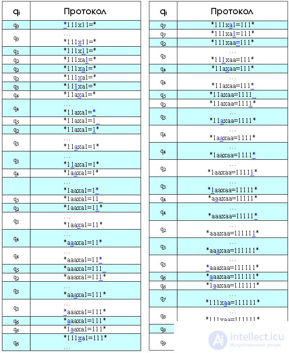
Multiply with MT 3 by 2 in the unit system. The protocol indicates the initial and final states of the MT, the initial configuration on the tape and the location of the machine head (underlined symbol).
Start. We are in the state q 0 , entered the data into the machine: * 111x11 = *, the machine head is located on the first character *.
1st step. We look at the table of rules that the machine will do, being in the state q 0 and above the “*” symbol. This rule from the 1st column of the 5th row is q 0 * → q 0 * R. This means that we move to the state q 0 (that is, do not change it), the symbol will become “*” (that is, it will not change) and move along the text “* 111x11 = *” entered by us to the right by one position (R), then is on the 1st character 1. In turn, the state q 0 1 (1st column 1st row) is processed by the rule q 0 1 → q 0 1R. That is, again just going to the right by 1 position. This happens until we become on the "x" symbol. And so on: we take the state (the index at q), take the character on which we stand (underlined character), connect them and look at the processing of the resulting combination according to the table of rules.
In simple words, the multiplication algorithm is as follows: we mark the 1st unit of the 2nd factor, replacing it with the letter “a”, and transfer the whole 1st factor to the equal sign. The transfer is performed by alternately replacing the units of the 1st factor by “a” and adding the same number of units at the end of the line (to the left of the rightmost “*”). Then we change all “a” to the multiplication sign “x” back by one. And the cycle repeats. Indeed, because A multiplied by B can be represented as A + A + A B times. We now mark the 2nd unit of the 2nd multiplier with the letter “a” and transfer the units again. When there are no units before the “=” sign, then multiplication is complete.
It can be said that the Turing machine is a simple linear memory computer that, according to formal rules, transforms input data using a sequence of elementary actions .
The elementary nature of actions lies in the fact that an action changes only a small piece of data in memory (in the case of a Turing machine, only one cell), and the number of possible actions is of course. Despite the simplicity of the Turing machine, it is possible to calculate everything that can be calculated on any other machine that performs calculations using a sequence of elementary actions. This property is called completeness .
One of the natural ways of proving that the computing algorithms that can be implemented on one machine can be implemented on another is imitating the first machine to the second.
Imitation is as follows. At the entrance to the second car, the description of the program (work rules) of the first car  and input
  which should have been received at the entrance of the first car. It is necessary to describe such a program (the rules of the second machine), so that as a result of the calculations on the output, the same thing turns out that the first machine would return if it received data .
As it was said, on the Turing machine it is possible to imitate (by setting the transition rules) all other performers, with the exception of competitive ones, in some way implement the step-by-step calculation process, in which each step of the calculation is quite elementary.
On a Turing machine, you can simulate a Post machine, normal Markov algorithms, and any program for ordinary computers that transforms input data into a weekend by some algorithm. In turn, on various abstract artists you can imitate the Turing Machine. The performers for whom this is possible are called Turing complete.
There are programs for ordinary computers that imitate the work of a Turing machine. But it should be noted that this imitation is incomplete, since there is an abstract endless ribbon in the Turing machine. An infinite data tape cannot be fully imitated on a computer with finite memory (total computer memory — RAM, hard disks, various external storage media, registers and processor caches, etc. — can be very large, but, nevertheless, always is finite).
Turing machine model allows extensions. Turing machines with an arbitrary number of tapes and multidimensional tapes with different constraints can be considered. However, all of these machines are Turing-complete and are modeled by a conventional Turing machine.
As an example of such information, consider the following theorem: For any Turing machine, there is an equivalent Turing machine running on a semi-infinite tape.
Consider the proof given by Yu. G. Karpov in the book “Automata Theory”. The proof of this theorem is constructive, that is, we give an algorithm by which an equivalent Turing machine with a declared property can be constructed for any Turing machine. First, we randomly number the cells of the working tape MT, that is, we define the new location of the information on the tape:

Then we renumber the cells, and we will assume that the symbol “*” is not contained in the MT dictionary:
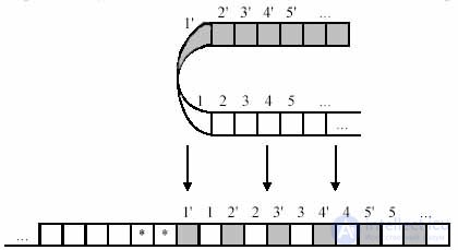
Finally, we change the Turing machine by doubling the number of its states, and change the read-write head shift so that in one group of states the machine’s operation would be equivalent to its operation in the shaded zone, and in the other group of states the machine would work as the original machine in the open zone. If the symbol '*' is encountered during the operation of the MT, then the read / write head has reached the zone boundary:
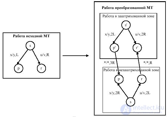
The initial state of the new Turing machine is set in one zone or another, depending on which part of the original tape the read / write head has in the original configuration. Obviously, to the left of the bounding markers "*" the tape in the equivalent Turing machine is not used.
Here, it should be noted that the term "semi-infinity" hardly has any intelligible meaning, since infinity divided into two is also infinity, which, in turn, has no "ends" by definition. Here, apparently, there was a terminological inaccuracy due to the fact that the definition of the Turing machine often uses the informal word "infinite in both directions".

Comments
To leave a comment
Theory of Automata
Terms: Theory of Automata