19.3. The flow of events. The simplest flow and its properties

Under the flow of events in probability theory is understood the sequence of events that occur one after another at some points in time. Examples include: call flow at a telephone exchange; the flow of devices in the household electrical network; the flow of registered letters arriving at the post office; flow of failures (malfunctions) of the electronic computer; the flow of shots directed at the target during the shelling, etc. The events forming the flow can be different in the general case, but here we will consider only the flow of homogeneous events differing only in the moments of their appearance. Such a stream can be depicted as a sequence of points. on the number axis (fig. 19.3.1), corresponding to the moments of occurrence of events.

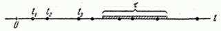
Fig. 19.3.1.

The flow of events is called regular if the events follow one after another at strictly defined intervals. Such a stream is relatively rare in real systems, but is of interest as a limiting case. A typical flow of queuing is typical for a queuing system.

Present we will look at event streams that have some particularly simple properties. To do this, we introduce a number of definitions.

1. The flow of events is called stationary, if the probability of a particular number of events falling on a time interval of length (fig. 19.3.1) depends only on the length of the section and does not depend on where exactly on the axis This plot is located.

2. The flow of events is called a flow without an after-action if, for any non-overlapping time segments, the number of events falling on one of them does not depend on the number of events falling on the others.

3. The flow of events is called ordinary if the probability of hitting an elementary segment two or more events are negligible compared to the probability of hitting a single event.

If the flow of events has all three properties (that is, is stationary, ordinary, and has no aftereffect), then it is called the simplest (or stationary Poisson) flow. The name "Poisson" is due to the fact that subject to conditions 1-3, the number of events falling on any fixed time interval will be distributed according to Poisson’s law (see 5.9).

Let us consider in more detail conditions 1-3, let us see what they correspond to for the flow of applications and due to what they can be violated.

1. The condition of stationarity is satisfied by the flow of applications, the probability characteristics of which do not depend on time. In particular, a constant density is characteristic for a stationary flow (the average number of applications per unit time). In practice, there are often application flows that (at least for a limited period of time) can be regarded as stationary. For example, a call flow at a city telephone exchange at a time interval from 12 to 13 hours can be considered stationary. The same flow for a whole day can no longer be considered stationary (at night the density of calls is much less than during the day). Note that this is the case with all the physical processes that we call “stationary”: in fact, they are all stationary only for a limited period of time, and the distribution of this area to infinity is just a convenient technique used to simplify the analysis. In many problems of queuing theory, it is of interest to analyze the operation of the system under constant conditions; then the problem is solved for the stationary flow of applications.

2. The condition of the absence of aftereffect — the most essential for the simplest flow — means that the applications enter the system independently of each other. For example, the flow of passengers entering the metro station can be considered a flow without an aftermath because the reasons for the arrival of an individual passenger at that particular moment and not at another time are usually not related to similar reasons for other passengers. However, the condition of the absence of aftereffect can be easily violated due to the appearance of such a dependence. For example, the flow of passengers leaving the metro station can no longer be considered a flow without an aftermath, since the exit times of passengers arriving by the same train are dependent on each other.

In general, it should be noted that the output flow (or the flow of served requests) leaving the queuing system usually has an after-effect, even if the input flow does not have it. To verify this, we consider a single-channel queuing system, for which the service time of one application is well defined and equals . Then, in the stream of serviced requests, the minimum time interval between requests leaving the system will be equal to . It is easy to verify that the presence of such a minimum interval inevitably leads to an aftereffect. Indeed, let it be known that at some point The service request has left the system. Then it can be argued with certainty that at any time lying within , the serviced order will not appear; hence, there will be a relationship between the numbers of events in non-overlapping areas.

The aftereffect inherent in the output stream must be taken into account if this stream is an input for any other queuing system (the so-called “multiphase service”, when the same request is sequentially transferred from system to system).

Note, by the way, that the simplest, at first glance, regular flow, in which events are separated from each other at regular intervals, is by no means the “simplest” in our sense of the word, since it has a pronounced aftereffect: the moments of appearance following each other Event related hard, functional addiction. It is because of the presence of aftereffect analysis of the processes occurring in the queuing system with a regular flow of applications, is much more difficult than with the simplest.

3. The condition of ordinary means that applications come one by one and not in pairs, triples, etc. For example, the flow of attacks to which an air target is exposed in the zone of action of fighter aircraft will be ordinary if the fighters attack the target alone, and will not be ordinary if fighters go to attack in pairs. The flow of clients entering the barber shop can be considered almost ordinary, which is not the case with the flow of clients heading to the registry office for marriage registration.

If in an extraordinary stream, applications are received only in pairs, only in triples, etc., then an extraordinary stream can easily be reduced to an ordinary stream; instead of a stream of individual applications, it is enough to consider a stream of pairs, triples, etc. It will be more difficult if each application can randomly turn out to be double, triple, etc. Then one has to deal with a stream of not homogeneous, but heterogeneous events.

In the following, for simplicity, we restrict ourselves to the consideration of ordinary flows.

Among the streams of events, the simplest flow generally plays a special role, to some extent analogous to the role of the normal law among other distribution laws. We know that by summing a large number of independent random variables, subordinate to virtually any distribution laws, we obtain a value that is approximately distributed according to the normal law. Similarly, one can prove that when summing up (mutual overlapping) of a large number of ordinary, stationary flows with practically any after-effect, a flow is obtained that is arbitrarily close to the simplest. The conditions that must be met for this are similar to the conditions of the central limit theorem, namely, the folding flows must have an approximately uniformly small effect on the sum.

Without proving this position and not even formulating mathematically the conditions with which the flows should satisfy, we illustrate it with elementary reasoning. Let there be a number of independent streams. (fig. 19.3.2). The "summation" of flows is that all moments of the occurrence of events are carried on the same axis. , as shown in Fig. 19.3.2.

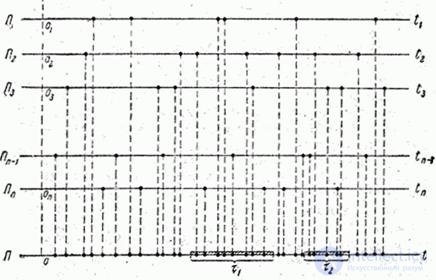
Fig. 19.3.2.

Suppose the threads they are comparable in their influence on the total flux (i.e., they have densities of the same order), and their number is rather large. Suppose, in addition, that these flows are stationary and ordinary, but each of them can have an aftereffect, and consider the total flow

(19.3.1)

on axis (fig. 19.3.2). Obviously, the flow must be stationary and ordinary, since each term has this property and they are independent. In addition, it is quite clear that with an increase in the number of terms, the aftereffect in the total flow, even if it is significant in separate flows, should gradually weaken. Indeed, consider on axis two non-overlapping segments and (fig. 19.3.2). Each of the points that fall into these segments may randomly belong to a particular stream, and as the proportion of points belonging to the same flow (and, therefore, dependent) must decrease, and the remaining points belong to different flows and appear on the segments independently of each other. It is natural to expect that with increasing the total flow will lose the aftereffect and approach the simplest.

In practice, it is usually enough to add 4-5 threads to get a stream with which you can operate as with the simplest.

The simplest flow plays a particularly important role in queuing theory. First, the simplest and closest to the simplest flows of applications are often found in practice (the reasons for this are set out above). Secondly, even with a bid flow that is different from the simplest one, it is often possible to obtain results that are satisfactory in accuracy by replacing the flow of any structure with the simplest with the same density. Therefore, let us take a closer look at the simplest flow and its properties.

Consider on the axis simple stream of events (fig. 19.3.3) as an unbounded sequence of random points.

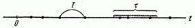
Fig. 19.3.3.

We select an arbitrary time interval of length . In chapter 5 ( 5.9) we have proved that under conditions 1, 2 and 3 (stationarity, absence of aftereffect and ordinaryness) the number of points falling on a segment distributed according to the Poisson law with the expectation

, (19.3.2)

Where - flux density (average number of events per unit of time).

Probability that for time will happen exactly events equal to

. (19.3.3)

In particular, the probability that the area will be empty (no events will occur) will be

. (19.3.4)

An important characteristic of the flow is the distribution of the length of the gap between adjacent events. Consider a random variable - the time interval between arbitrary two neighboring events in the simplest flow (Fig. 19.3.3) and find its distribution function

.

Let us turn to the probability of the opposite event.

.

This is the probability that the length of time starting at the moment the appearance of one of the events in the stream, none of the subsequent events will appear Since the simplest flow does not have an after-effect, the presence at the beginning of the segment (at the point ) some event does not affect the likelihood of those or other events in the future. Therefore, the probability can be calculated by the formula (19.3.4)

,

from where

. (19.3.5)

Differentiating, we find the distribution density

. (19.3.6)

The distribution law with a density (19.3.6) is called the exponential law, and the quantity - its parameter. Density chart presented in fig. 19.3.4.

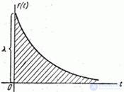
Rice 19.3.4.

The exponential law, as we will see later, plays a large role in the theory of discrete random processes with continuous time. Therefore, we consider it in more detail.

Find the expected value distributed by exponential law:

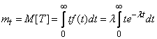
or, integrating in parts,

. (19.3.7)

Variance of magnitude equals

,

from where

, (19.3.8)

. (19.3.9)

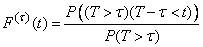
Let us prove one remarkable property of the exponential law. It consists in the following: if the time span, distributed according to the exponential law, has already lasted for some time then it does not affect the distribution of the rest of the gap: it will be the same as the distribution of the entire gap .

For proof, consider a random time span. with distribution function

(19.3.10)

and suppose that this gap has been going on for some time i.e. an event occurred . Under this assumption, we find the conditional distribution law for the remaining part of the interval. ; denote it

. (19.3.11)

Let us prove that the conditional distribution law does not depend on and is equal to . In order to calculate first we find the probability of the product of two events

and .

By the probability multiplication theorem

,

from where

.

But the event tantamount to an event whose probability is equal

.

On the other hand,

,

Consequently,

,

where, according to the formula (19.3.10), we get

,

Q.E.D.

So we proved that if the time span distributed according to the exponential law, then any information about how long this gap has already passed does not affect the law of distribution of the remaining time. It can be proved that the exponential law is the only one possessing such a property. This property of the exponential law is, in essence, another formulation for the “absence of aftereffect”, which is the basic property of the simplest flow.