Lecture
The assumptions about the Poisson nature of the flow of requests and the exponential distribution of service time are valuable in that they allow the use of the apparatus of so-called Markovian random processes in the theory of mass service.
A process that takes place in a physical system is called a Markov process (or a process without an after-effect), if for each time point the probability of any state of the system in the future depends only on the state of the system at the moment  and does not depend on how the system came to this state.
Consider an elementary example of a Markov random process. Abscissa axis  point randomly moves
  . At the moment of time
  point is at the origin
  and stays there for one second. A second later, a coin rushes; if the coat of arms fell - point moves one unit of length to the right, if the digit is to the left. After a second, the coin rushes back and the same random movement is made, etc. The process of changing the position of a point (or, as they say, “wandering”) is a random process with discrete time
  and a countable set of states

A diagram of possible transitions for this process is shown in Fig. 19.7.1.

Fig. 19.7.1.
Let us show that this process is Markov. Indeed, imagine that at some point in time  the system is, for example, able
  - one unit to the right of the origin. Possible positions of a point in a unit of time will be
  and
and  with probabilities 1/2 and 1/2; after two units -
  , ,
, ,  with probabilities 1/4, ½, 1/4 and so on. Obviously, all these probabilities depend only on where the point is at the moment. , and completely independent of how she came there.
Consider another example. There is a technical device consisting of elements (details) types  and
and  with different durability. These elements can fail at random times and independently of each other. The proper operation of each element is absolutely necessary for the operation of the device as a whole. The uptime of the element is a random variable distributed according to the exponential law; for items of type and the parameters of this law are different and equal respectively
  and
and  . In the event of a device failure, measures are taken immediately to identify the causes and the detected faulty element is immediately replaced with a new one. The time required to restore (repair) the device is distributed exponentially with the parameter
  (if an element of type has failed ) and
  (if an element of type has failed ).
In this example, the random process occurring in the system is a Markov process with continuous time and a finite set of states:
- all elements are intact, the system works,
- defective item type , the system is being repaired,
- defective item type The system is being repaired.
The scheme of possible transitions is given in fig. 19.7.2.
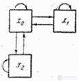
Fig. 19.7.2.
Indeed, the process has a Markov property. Let for example, at the moment system is able to (OK) Since the uptime of each element is indicative, the time of failure of each element in the future does not depend on how long it has been working (when delivered). Therefore, the probability that the system will remain in the future or leave it does not depend on the "background" of the process. Suppose now that at the moment system is able to (defective item type ). Since the repair time is also indicative, the probability of the end of the repair at any time after does not depend on when the repair began and when the rest (serviceable) elements were delivered. Thus, the process is Markov.
Note that the exponential distribution of the element operation time and the exponential distribution of the repair time are essential conditions, without which the process would not be Markovian. Indeed, let us suppose that the time of a good operation of an element is distributed not according to the exponential law, but according to some other - for example, according to the law of uniform density in the area  . This means that each item with a guarantee of working time.
  , and on the plot from before
  can fail at any time with the same probability density. Suppose that at some point in time The item is working properly. Obviously, the likelihood that an element will fail at some time in the future depends on how long the element is delivered, that is, it depends on history, and the process will not be Markovian.
The situation is the same with the repair time.  ; if it is not exponential and the element is at the moment repaired, the remaining repair time depends on when it started; the process will not be Markov again.
In general, the exponential distribution plays a special role in the theory of Markov random processes with continuous time. It is easy to verify that in a stationary Markov process the time during which the system remains in any state is always distributed according to the exponential law (with a parameter depending, generally speaking, on this state). Indeed, suppose that at the moment system is able to  and before that it had been there for some time. According to the definition of the Markov process, the probability of any event in the future does not depend on the prehistory; in particular, the probability that the system will leave the state for a time
  , should not depend on how much time the system has already spent in this state. Therefore, the time the system is in should be distributed according to the indicative law.
In the case when the process proceeding in a physical system with a countable set of states and continuous time is Markov, this process can be described using ordinary differential equations, in which the unknown functions are the probabilities of the states  . The compilation and solution of such equations will be demonstrated in the following
  on the example of the simplest queuing system.

Comments
To leave a comment
Queuing theory
Terms: Queuing theory