19.10. Queuing system with waiting

A queuing system is called a system with a wait, if an application that has made all channels busy becomes in a queue and waits until a channel becomes free.

If the waiting time for an application in the queue is not limited by anything, then the system is called a “clean system with waiting”. If it is limited by some conditions, then the system is called a “mixed type system”. This is an intermediate case between a clean system with failures and a clean system with a wait.

For practice, the most interesting are systems of mixed type.

The restrictions imposed on waiting can be of various types. It often happens that the restriction is imposed on the waiting time of the application in the queue; it is considered to be restricted from above for a period of time. which can be either strictly defined or random. At the same time, only the waiting time in the queue is limited, and the started service is completed, regardless of how long the waiting lasted (for example, the client at the barbershop sitting in the chair usually does not go to the end of the service). In other tasks it is more natural to impose a restriction not on the waiting time in the queue, but on the total time the application is in the system (for example, an air target can stay in the firing zone only for a limited time and leave it regardless of whether the shelling is over or not). Finally, it is possible to consider such a mixed system (it is closest to the type of commercial enterprises selling non-essential items), when an application is placed in a queue only if the queue length is not too long. Here the limit is imposed on the number of applications in the queue.

In systems with anticipation, the so-called “queue discipline” plays a significant role. Pending applications can be called up for service both in the order of the queue (earlier arrived earlier and serviced), and in a random, unorganized order. There are queuing systems "with benefits", where some applications are served preferentially over others ("generals and colonels out of turn").

Each type of system with expectation has its own characteristics and its own mathematical theory. Many of them are described, for example, in V. V. Gnedenko’s book Lectures on the Theory of Queuing Theory.

Here we dwell only on the simplest case of a mixed system, which is a natural generalization of the Erlang problem for a system with refusals. For this case, we derive differential equations similar to the Erlang equations, and formulas for the probabilities of states in the steady state, similar to the Erlang formulas.

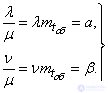
Consider a mixed queuing system with channels under the following conditions. At the input of the system comes the simplest flow of applications with a density . Service time for one application - indicative, with parameter . An application that has made all channels busy is queued and is waiting for service; waiting time is limited to some time ; if the application is not accepted for servicing before the expiration of this period, it leaves the queue and remains unattended. Waiting time we will be considered random and distributed according to the exponential law

,

where is the parameter - the reciprocal of the average waiting time:

; .

Parameter completely analogous to the parameters and application flow and release flow. It can be interpreted as the density of the "flow of departures" of the application, standing in line. Indeed, let us imagine an application that only does what becomes in the queue and waits in it until the waiting period ends. , then leaves and immediately queued up again. Then the “flow of withdrawals” of such an application from the queue will have a density .

Obviously when the mixed type system becomes a clean system with failures; at it turns into a clean system with anticipation.

Note that with the exponential law of waiting time distribution, the system capacity does not depend on whether requests are serviced in a queue or in a random order: for each application, the law of distribution of the remaining waiting time does not depend on how long the request was already in the queue.

Due to the assumption of the Poisson character of all event flows that lead to changes in the states of the system, the process proceeding in it will be Markovian. We write the equations for the probabilities of the states of the system. To do this, first of all, we list these states. We will number them not by the number of channels occupied, but by the number of requests related to the system. The application will be called "system-related" if it is either in a state of service or waiting in line. Possible system states will be:

- no channel is busy (no queue),

- exactly one channel is busy (no queue),

………

- busy exactly channels (no queue)

………

- all busy channels (no queue)

- all busy channels, one application is in the queue,

………

- all busy channels, applications are waiting in line

………

Number of applications standing in line in our conditions can be arbitrarily large. Thus, the system has an infinite (albeit countable) set of states. Accordingly, the number of differential equations describing it will also be infinite.

Obviously, the first differential equations will not differ from the corresponding Erlang equations:

The difference between the new equations and the Erlang equations will begin when . Indeed, in the state system with failures can only go from the state ; as for the system with the expectation, it can go into a state not only from but also from (all channels are busy, one application is in the queue).

Let's make the differential equation for . Fix the moment and find - the probability that the system is at the moment will be able to . This can be done in three ways:

1) at the moment the system was already able and in time did not come out of it (not a single application came and not a single channel was released);

2) at the moment the system was able to and in time moved to state (one application has arrived);

3) at the moment the system was able to (all channels are busy, one application is in the queue), and during moved to (either one channel was released and the queued application occupied it, or the queued application went away due to the expiration of the term).

We have:

,

from where

.

Calculate now at any - the probability that at the moment everything channels will be busy and smooth applications will stand in line. This event can again be realized in three ways:

1) at the moment the system was already able and in time this state has not changed (it means that not a single application has arrived, not a single drop has been released and not a single one queued applications did not go away);

2) at the moment the system was able to and in time moved to state (i.e. one application has arrived);

3) at the moment the system was able to and in time moved to state (for this, either one of the channels must be freed, and then one of queuing applications will occupy it, or one of the queuing applications must leave due to the expiration).

Consequently:

,

from where

.

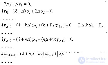
Thus, for the state probabilities, we have obtained a system of infinite number of differential equations:

(19.10.1)

Equations (10/19/1) are a natural generalization of the Erlang equations to the case of a mixed-type system with a limited waiting time. Options in these equations can be both constant and variable. When integrating system (19.10.1), it must be taken into account that although theoretically the number of possible states of the system is infinite, in practice the probabilities with increasing become negligible, and the corresponding equations can be discarded.

We derive formulas similar to the Erlang formulas for the probabilities of the system states at the steady state of service (with ). From equations (10/19/1), assuming all constant, and all derivatives - equal to zero, we get a system of algebraic equations:

(19.10.2)

They need to attach the condition:

. (19.10.3)

Let us find the solution of the system (19.10.2).

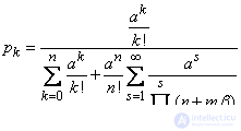
For this, we apply the same technique that we used in the case of a system with failures: solve the first equation with respect to we will substitute in the second, etc. For any as in the case of a system with failures, we get:

. (19.10.4)

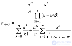
We turn to the equations for . In the same way we get:

,

,

and generally for any

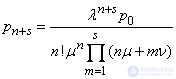. (19.10.5)

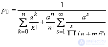
In both formulas (19.10.4) and (19.10.5), the probability . We define it from the condition (19.10.3). Substituting into it the expressions (19.10.4) and (19.10.5) for and , we get:

,

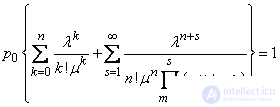from where

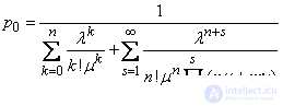. (19.10.6)

Let's transform expressions (19.10.4), (19.10.5) and (19.10.6), entering in them instead of densities and "Reduced" density:

(19.10.7)

Options and express, respectively, the average number of applications and the average number of requests left in a queue, falling on the average service time of a single application.

In the new notation of the formula (19.10.4), (19.10.5) and (19.10.6) will take the form:

; (19.10.8)

; (19.10.9)

. (10/19/10)

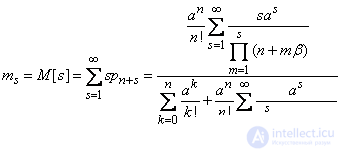
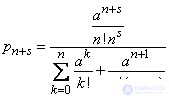
Substituting (19.10.10) into (19.10.8) and (19.10.9), we obtain the final expressions for the probabilities of the system states:

; (10/19/11)

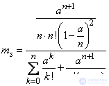
. (10/19/12)

Knowing the probabilities of all system states, one can easily determine other characteristics of interest to us, in particular, the probability that the application leaves the system unattended. We define it from the following considerations: at steady state, the probability the fact that an application leaves the unserved system is nothing but the ratio of the average number of applications leaving the queue per unit of time to the average number of applications received per unit of time. Find the average number of applications leaving the queue per unit of time. To do this, we first calculate the expectation the number of applications in the queue:

. (10/19/13)

To obtain , need to multiply by the average "density of departures" of one application and divided by the average density of applications i.e. multiply by a factor

.

We get:

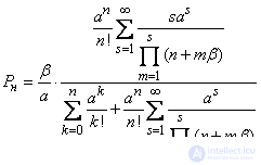. (10/19/14)

The relative capacity of the system is characterized by the probability that an application that has entered the system will be served:

.

Obviously, the system bandwidth with the expectation, with the same and , будет всегда выше, чем пропускная способность системы с отказами: в случае наличия ожидания необслуженными уходят не все заявки, заставшие каналов занятыми, а только некоторые. Пропускная способность увеличивается при увеличении среднего времени ожидания .

Непосредственное пользование формулами (19.10.11), (19.10.12) и (19.10.14) несколько затруднено тем, что в них входят бесконечные суммы. Однако члены этих сумм быстро убывают.

Посмотрим, во что превратятся формулы (19.10.11) и (19.10.12) при and . Obviously, when система с ожиданием должна превратиться в систему с отказами (заявка мгновенно уходит из очереди). Indeed, with формулы (19.10.12) дадут нули, а формулы (19.10.11) превратятся в формулы Эрланга для системы с отказами.

Рассмотрим другой крайний случай: чистую систему с ожиданием .In such a system, applications do not leave the queue at all, and therefore : each application will wait for service sooner or later. But in a clean system with waiting, there is not always a limit stationary mode when .It can be proved that such a regime exists only if , that is, when the average number of requests per service time of one application does not go beyond the limits of the -channel system. If , the number of applications in the queue will increase unlimitedly over time.

Let's pretend that , and find the limit probabilities for a pure system with expectation. To do this, we put in formulas (19.9.10), (19.9.11) and (19.9.12) . We get:

,

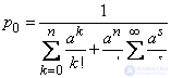or, summing up the progression (which is only possible with ),

. (10/19/15)

From here, using the formulas (10/19/08) and (10/19/9), we find

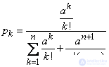(10/19/16)

and likewise for

. (10/19/17)

The average number of applications in the queue is determined from the formula (10/19/13) with :

. (10/19/18)

Example 1. At the input of a three-channel system with an unlimited waiting time comes the simplest flow of applications with density (applications per hour). Average service time for one application minDetermine if steady state maintenance exists; if yes, then find the probabilities , the probability of having a queue and the average queue length .

Decision. We have ; . Because , steady state exists. By the formula (10/19/16) we find

; ; ; .

The likelihood of a queue:

.

The average queue length by the formula (10/19/18) will be

(application).