Lecture
The following types of signals are distinguished, which correspond to certain forms of their mathematical description.
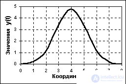
An analog signal is a continuous function of a continuous argument, i.e. defined for any value of the arguments. Sources of analog signals, as a rule, are physical processes and phenomena that are continuous in the dynamics of their development in time, in space or in any other independent variable, while the recorded signal is similar (“similar”) to the process that generates it. An example of a mathematical record of a signal: y (t) = 4.8 exp [- (t-4)2/2.8]. An example of a graphical display of this signal is shown in Fig. 1, while both the function itself and its arguments can take any values within some intervals y1Ј yЈy2, t1Ј t Ј t 2 . If the intervals of the signal values or the independent variables are not limited to, by default, they are set from - ¥ to + ¥ . The set of possible signal values forms a continuum - a continuous space in which any signal point can be determined up to infinity. Examples of signals that are analog in nature are changes in the strength of the electric, magnetic, electromagnetic field in time and space.
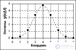
A discrete signal by its values is also a continuous function, but determined only by the discrete values of the argument. According to the set of its values, it is finite (countable) and is described by a discrete sequence of samples (samples) y (nDt), where y1Ј yЈy2,Dt is the interval between samples (interval or sampling step, sample time), n = 0, 1, 2, ..., N. The reciprocal of the sampling step: f = 1 /Dt is called the sampling frequency. If a discrete signal is obtained by sampling an analog signal, then it is a sequence of samples, the values of which are exactly equal to the values of the original signal along the coordinates n D t.
An example of sampling the analog signal shown in Fig. 1 is shown in Fig. 1.2.2. When D t = const (uniform data sampling), the discrete signal can be described by the abbreviated notation y (n). In the technical literature, in the notation of discretized functions, the former indices of the arguments of analog functions are sometimes left, enclosing the latter in square brackets - y [ t ]. With non-uniform sampling of the signal, the designations of discrete sequences (in text descriptions) are usually enclosed in curly braces - {s (t i )}, and the sample values are given in the form of tables indicating the values of the coordinates t i . For numerical sequences (uniform and non-uniform), the following numerical description also applies: s (ti ) = {a 1 , a 2 , ..., a N }, t = t 1 , t 2 , ..., t N . Examples of discrete geophysical signals are the results of vertical electrical sounding (discrete distance of current electrodes), profiles of geochemical sampling, etc.
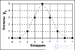
A digital signal is quantized in value and discrete in argument. It is described by the quantized lattice function yn= Qk[y (nDt)], where Qkis the quantization function with the number of quantization levels k, and the quantization intervals can be either uniformly distributed or nonuniform, for example, logarithmic ... A digital signal is set, as a rule, in the form of a discrete series of numerical data - a numeric array of sequential values of the argument whenDt = const, but in the general case, the signal can also be set in the form of a table for arbitrary values of the argument.
По существу, цифровой сигнал по своим значениям (отсчетам) является формализованной разновидностью дискретного сигнала при округлении отсчетов последнего до определенного количества цифр, как это показано на рис 1.2.3. Цифровой сигнал конечен по множеству своих значений. Процесс преобразования бесконечных по значениям аналоговых отсчетов в конечное число цифровых значений называется квантованием по уровню, а возникающие при квантовании ошибки округления отсчетов (отбрасываемые значения) – шумами (noise) или ошибками (error) квантования (quantization).
In digital data processing systems and computers, the signal is always presented with an accuracy of up to a certain number of digits, and, therefore, is always digital. Taking these factors into account, when describing digital signals, the quantization function is usually omitted (it is assumed uniform by default), and the rules for describing discrete signals are used to describe signals. As for the form of digital signals in storage, transmission and processing systems, as a rule, they are combinations of short unipolar or bipolar impulses of the same amplitude, which are encoded in a binary code with a certain number of numerical digits the numerical sequences of signals (data arrays).
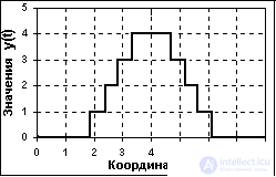
In principle, analog signals recorded by the corresponding equipment (Fig. 1.2.4), which are usually called discrete-analog signals, can also be quantized in their values. But it makes no sense to separate these signals into a separate type - they remain analog piecewise continuous signals with a quantization step, which is determined by the permissible measurement error.
Most of the signals that have to be dealt with in processing geophysical data are analog in nature, sampled and quantized due to the methodological features of measurements or technical features of registration, i.e. converted to digital signals. But there are also signals that initially belong to the digital class, such as counting the number of gamma quanta recorded at successive time intervals.

Comments
To leave a comment
Signal and linear systems theory
Terms: Signal and linear systems theory