Lecture
Forms of mathematical display of signals, especially at the stages of their primary registration (detection) and in direct problems of describing geophysical fields and physical processes, as a rule, reflect their physical nature. However, the latter is not mandatory and depends on the measurement technique and technical means for detecting, converting, transmitting, storing and processing signals. At different stages of the processes of obtaining and processing information, both the material representation of signals in recording and processing devices and the forms of their mathematical description in the analysis of data can be changed by appropriate conversion operations of the signal type.
The discretization operation converts analog signals (functions), continuous by argument, into a function of instantaneous values of signals by a discrete argument. Discretization is usually performed with a constant step in the argument (uniform discretization), while s (t)10s (nDt), where the values of s (nDt) are samples of the function s (t) at times t = nDt, n = 0, 1, 2, ..., N. The frequency at which the analog signal is measured is calledthe sampling rate. In the general case, the grid of samples by the argument can be arbitrary, such as, for example, s (t)10s (tk), k = 1, 2,…, K, or set according to a certain law. As a result of sampling, a continuous ( analog ) signal is converted into a sequence of numbers.
The operation of restoring an analog signal from its discrete representation is the opposite of sampling and is essentially data interpolation.
Sampling of signals can lead to a certain loss of information about the behavior of signals in the intervals between samples. However, there are conditions determined by the Kotelnikov-Shannon theorem, according to which an analog signal with a limited frequency spectrum can be converted into a discrete signal without information loss, and then absolutely accurately restored from the values of its discrete samples.
As you know, any continuous function can be expanded on a finite segment in a Fourier series, i.e. is presented in spectral form - as the sum of a series of sinusoids with multiple (numbered) frequencies with specific amplitudes and phases. For relatively smooth functions, the spectrum decreases rapidly (the coefficients of the modulus of the spectrum rapidly tend to zero). To represent "jagged" functions, with discontinuities and "kinks", sinusoids with high frequencies are needed. A signal is said to have a limited spectrum if, after a certain frequency F, all the spectral coefficients are zero, i.e. the signal is represented as a finite sum of the Fourier series.
The Kotelnikov-Shannon theorem establishes that if the signal spectrum is limited by the frequency F, then after sampling the signal with a frequency of at least 2F, it is possible to restore the original continuous signal from the received digital signal absolutely accurately. To do this, you need to interpolate the digital signal "between samples" by a special function (Kotelnikov-Shannon).
In practice, this theorem is of great importance. For example, it is known that the range of audio signals perceived by a person does not exceed 20 kHz. Therefore, by sampling recorded audio signals with a frequency of at least 40 kHz, we can accurately reconstruct the original analog signal from its digital samples, which is what CD players do to restore sound. The audio signal sampling rate for CD recording is 44100 Hz.
The operation of quantization or analog-to-digital conversion (ADC; English term Analog-to-Digital Converter, ADC) consists in converting a discrete signal s (tn) into a digital signal s (n) = sn" s (tn), n = 0, 1, 2, .., N, usually encoded in a binary number system. The process of converting signal samples into numbers is called quantization, and the resulting loss of information due to rounding is called quantization error or quantization noise.
When converting an analog signal directly to a digital signal, sampling and quantization are combined.
The operation of digital-to-analog conversion (DAC; Digital-to-Analog Converter, DAC) is the opposite of the quantization operation, while the output registers either a discrete-analog signal s (tn), which has a stepped shape (Fig. 1.2.4), or directly analog signal s (t), which is reconstructed from s (tn), for example, by smoothing.
Since the signal quantization is always performed with a certain and fatal error (maximum - up to half of the quantization interval), the ADC and DAC operations are not mutually inverse with absolute accuracy.
Aliasing. What happens if the spectrum of the analog signal was unlimited or had a frequency higher than the sampling rate?
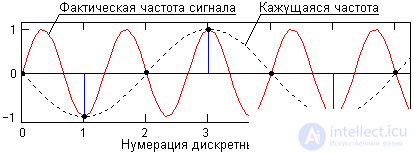
Suppose that when recording the acoustic signal of an orchestra in a room from some device, an ultrasonic signal with a frequency of 30 kHz is present. Recording is performed by sampling the microphone output at a typical frequency of 44.1 kHz. When listening to such a recording using a DAC, we will hear a noise signal at a frequency of 30 - 44.1 / 2 " 8 kHz. The reconstructed signal will look as if the frequencies lying above half of the sampling frequency were "mirrored" from it to the lower part of the spectrum and added up with the harmonics present there. This is the so-called effect of the appearance of false (apparent) frequencies.(aliasing). The effect is similar to the well-known effect of reverse rotation of the wheels of a car on cinema and TV screens, when their rotation speed begins to exceed the frame rate. The nature of the effect can be clearly seen in Fig. 1.2.5. Similarly, all high-frequency noise present in the original analog signal is "reflected" from the sampling frequency into the main frequency range of discrete signals.
To prevent aliasing, the sampling rate should be increased or limit the signal spectrum before digitizing filters low frequency ( LF filters , low-pass filters ), which is passed unchanged all frequencies below a predetermined, frequency and suppress a signal above the set. This cutoff frequency is called the cutoff frequency ( cutoff frequency ) filter. The cutoff frequency of the anti-aliasing filters is set to half the sampling frequency. An anti-aliasing filter is almost always built into real ADCs.
The graphic display of signals is well known and does not require special explanations. For one-dimensional signals, a graph is a collection of pairs of values {t, s (t)} in a rectangular coordinate system (Fig. 1.2.1 - 1.2.4). When graphically displaying discrete and digital signals, either the method of direct discrete segments of the corresponding scale length over the axis of the argument is used, or the method of the envelope (smooth or broken) by the sample values. Due to the continuity of geophysical fields and, as a rule, the secondary nature of digital data obtained by sampling and quantizing analog signals, the second method of graphic display will be considered the main one.
Test signals (testsignal). As test signals, which are used in modeling and research of data processing systems, signals of the simplest type are usually used: harmonic sine-cosine functions, delta function and unit hop function.
Delta function or Dirac function. By definition, a delta function is described by the following mathematical expressions (collectively):
d (t- t ) = 0 at t # t ,
 d (t- t ) dt = 1.
The function d (t - t ) is not differentiable, and has a dimension inverse to the dimension of its argument, which directly follows from the dimensionlessness of the integration result. The value of the delta function is zero everywhere except at point t , where it is an infinitely narrow pulse with an infinitely large amplitude, while the area of the pulse is 1.
The delta function is a useful mathematical abstraction. In practice, such functions cannot be implemented with absolute precision, since it is impossible to realize a value equal to infinity at the point t = t on an analog time scale, i.e. determined in time also with infinite precision. But in all cases, when the pulse area is equal to 1, the pulse duration is rather short, and during its operation at the input of any system, the signal at its output practically does not change (the system's response to the pulse is many times greater than the pulse duration), the input signal can be considered a unit impulse function with delta-function properties.
For all its abstractness, the delta function has a definite physical meaning. Imagine a rectangular pulse signal P (t- t ) with a duration q , the amplitude of which is 1 / q , and the area, respectively, is 1. When the value of the duration q decreases , the pulse, decreasing in duration, retains its area equal to 1, and increases in amplitude ... The limit of such an operation at q 10 0 is called delta - impulse. This signal d (t- t ) is concentrated in one coordinate point t = t, the specific amplitude value of the signal is not determined, but the area (integral) remains equal to 1. This is not the instantaneous value of the function at the point t = t , but the impulse (impulse of force in mechanics, impulse of current in electrical engineering, etc.) is a mathematical model short acting with a value of 1.
The delta function has a filtering property . Its essence lies in the fact that if the delta function d (t- t ) enters the integral of any function as a factor, then the result of integration is equal to the value of the integrand at point t of the location of the delta pulse, i.e.:
f (t) d (t- t ) dt = f ( t ).
Integration in this expression can be limited to the immediate vicinity of the point t .
The single hop function or Heaviside function is sometimes also called the enable function. Complete mathematical expression of the function:
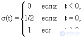
When simulating signals and systems, the value of the jump function at the point t = 0 is very often taken equal to 1, if this is not of fundamental importance.
The single hop function is used to create mathematical models of signals of finite duration. When multiplying any arbitrary function, including a periodic one, by a rectangular pulse formed from two successive functions of a unit jump
s (t) = s (t) - s (tT),
a section on the 0-T interval is cut out from it, and the function values outside this interval are reset to zero.
Kronecker function. For discrete and digital systems, the signal argument resolution is determined by its sampling intervalDt. This allows a discrete integral analogue of the delta function to be used as a unit impulse - the unit counting functiond(kDt-nDt), which is equal to 1 at the coordinate point k = n, and zero at all other points. The functiond(kDt-nDt) can be defined for any values ofDt = const, but only for integer values of coordinates k and n, since there are no other numbers of samples in discrete functions.
The mathematical expressions d (t- t ) and d (k D t-n D t) are also called the Dirac and Kronecker impulses. However, using this terminology, let us not forget that these are not just single impulses at the coordinate points t and n D t, but full-scale impulse functions that determine both the values of the impulses at certain coordinate points and zero values for all other coordinates, in the limit from - ¥ to ¥ .

Comments
To leave a comment
Signal and linear systems theory
Terms: Signal and linear systems theory